The Overlapping Generations model, often called the “OLG model”, is a cornerstone macroeconomics model that does away with one nearly universal assumption. Similarly to the Solow-Swan model, it’s often used to describe the overall economy, and can be used to find an optimal growth path for an economy.

Many economic models, particularly those taught in introductory courses, include a “representative agent” assumption. This means we assume that economic agents (or households) across the economy are all the same. This greatly simplifies the math and allows us to reach, and discuss, the implications of each model without getting lost in pages of arcane symbols.

However, this is the key assumption that the OLG model does away with. Instead, in the OLG model, there are two different kinds of agents, usually called “young” and “old”. This has far-reaching implications for economic outcomes, as we will soon see.

Introducing the basic OLG model

One of the model’s main focuses is studying how heterogeneous agents affect economic outcomes, particularly with regard to phenomena such as social security systems and public debt accumulation. To accomplish this, the OLG model makes a simple but elegant assumption.

This simple assumption is: in each time period, there is a young generation and an old generation. The young generation works and earns income, and chooses to maximize their utility while saving some money for retirement. The old generation does not work and has no income. Instead, they consume based on the savings they set aside in the prior time period (when they were young workers).

As a note, the OLG model is measured in “discrete” time. This means that there is not a continuous flow of time: rather, each sequential point in time is distinct from the rest. For example, in discrete time 1976 and 1977 could both be time periods, but “halfway through 1976” would not make sense.

We represent each point of discrete time by t. In each time period, new young agents appear – they either immigrate or are born – and young agents from the previous period become old. Agents live for two periods, such that each is young in one period and old in the next. We further assume that the population grows larger each period.

Population growth is therefore modeled by: L_t+1 = (1+n)L_t, where n is the rate of population growth and L_t is the size of the young generation. Notice that in each time period, the old generation can be represented by L_t-1, since the previous period’s young generation becomes the current period’s old generation (similarly, L_t+1 represents the next period’s young generation). We assume that each young agent supplies 1 unit of labor, and each old agent supplies 0 units of labor. Because of this, old agents don’t appear directly in the production function!

Output and the production function are modeled by Y_t = F(K_t,A_tL_t), where Y_t represents economic output (and therefore also income) in each time period, and the term F(K_t,A_tL_t) shows that we have an unknown production function F containing three important variables: Kt, At, and L_t.

Kt is capital in each period. At represents the level of technology while L_t was already defined as the amount of young agents in each period. Since we assumed that young agents supply 1 unit of labor and old agents supply 0, L_t also represents the labor force. A_tL_t is therefore the productivity of labor, which can be increased by adding workers or increasing the level of technology.

A few more assumptions must be made to complete the outline of the model. 

• Economic output is homogenous: all goods are the same. Further, this single good can be used for both production and consumption.
• Markets are perfectly competitive, which lets us normalize prices to 1 and ignore the effects of money.
• There is no foreign trade: this economy is in autarky.
• There are constant returns to scale in production.
• Economic agents are rational and have perfect information.

There’s technically one more important assumption we need in order to set up the model. Suppose that agents choose to take out a loan to finance all of their consumption in the first period of life, and take out more loans in the second period to cover the interest they must pay back. In the OLG model, this could create an infinite cycle of debt being used to finance everything, which is nonsensical.

We formally assume that this does not happen, so that the model can work properly without yielding this unrealistic solution. This is known as the “no Ponzi game solution” assumption.

Analyzing firm behavior

As with the Solow-Swan model, markets are assumed to be perfectly competitive. This means that firms make zero profits in equilibrium, and prices can be normalized to 1 and largely ignored.

In the basic OLG model, firms solve the following optimization problem:

Π = Y_t – w_tL_t – r_tK_t

where Π, the Greek capital letter pi, is the symbol typically used to represent profit in economics. This is the firm’s profit equation: income Y_t minus the total cost of paying labor w_tL_t minus the total cost of renting capital r_tK_t.

Income is determined by the production function we choose. Let’s stick with the general form F(K_t,A_tL_t) as most economics courses do. This transforms the profit equation into:

Π = F(Kt,A_tL_t) – w_tL_t – r_tK_t

We could account for depreciation 𝛿 by subtracting the term 𝛿Kt from the above as well. Either way, the first-order conditions for this profit equation reveal the firm’s solution. Taking the partial derivative with respect to labor L_t and capital K_t yield the following familiar conditions:

𝝏Π/𝝏L_t = w_t = marginal product of labor (MPL)

𝝏Π/𝝏K_t = r_t = marginal product of capital (MPK); with depreciation included, this becomes r_t – 𝛿

These results show clearly that firms make zero profits in this perfectly competitive equilibrium.

Knowing how firms behave allows us to get into the more interesting and unique parts of the OLG model: household behavior, and later, government policy.

Setting up the household optimization problem

As usual, in the OLG model households are composed of rational economic agents that maximize their utility subject to a budget constraint. Unlike usual, recall that we’re assuming that there are two types of agents – young and old.

Typically in the OLG model, it’s assumed that households own capital and rent it to firms. While this may seem unrealistic, the model’s outcome is the same when we assume that firms own capital, but must pay their shareholders (who are households). Thus, it’s simpler to stick to the former assumption rather than the latter.

The young generation earns income w_t, and saves a portion of it for time t+1 when they will be old. They seek to maximize utility in both periods subject to their budget constraint of lifetime earnings, as follows:

maximize U(c_Y,c_O) subject to two budget constraints:

1. w_t = c_Y + s_t
2. c_O = (1 + r_t)s_t

where U(c_Y,c_O) represents a utility function U with two major variables, consumption when young (c_Y) and consumption when old (co). The budget constraints show two important things. First, income w_t can be used for either consumption in the first period c_Y or savings s_t, which becomes income for the second period. Next, consumption in the second period c_O equals the rate of return on savings from the first period.

We can use this first budget constraint to reach the following Lagrangian optimization* problem:

max_c U(c_Y,c_O) – λ(w_t – (c_Y + s_t))

*A note for advanced students: the Lagrangian problem here often becomes a “Hamiltonian” in advanced economics classes. This is a similar technique that’s better suited to analyzing behavior over time.

But, this equation is incomplete – and not just because we haven’t used budget constraint number two yet.

Consider that young people making savings decisions don’t necessarily value consumption in each period equally. Someone who is very impatient would likely consume more in the first period, and have less left over in the second. Meanwhile, a very patient person would likely sacrifice some consumption in the present to save more for the future.

To account for this behavior, we need to introduce a new parameter 𝜌 to represent time preferences. 𝜌 is often described in economics courses as “(im)patience” (some courses may use 𝛽 instead). With 𝜌, we can split U(c_Y,c_O) into two components: U(c_Y,c_O) = u(c_Y) + 𝜌u(c_O). This shows that a young person making budgeting decisions must choose between utility now and utility later (which is modified by their (im)patience).

One of the interesting conclusions of the OLG model is the following: 𝜌 can cause the economy to reach Pareto inefficient equilibria! This is called “dynamic inefficiency”. In short, when people’s preferred rate of savings is different from the socially optimal level of savings, the economy may grow in a way that is Pareto inefficient. This means there is a Pareto improvement available to reach a strictly better equilibrium.

We’ll see later how fiscal policy can (theoretically) help prevent dynamic inefficiency. First, we must account for these time preferences in the utility maximization problem. The household optimization problem becomes:

max_c u(c_Y) + 𝜌u(c_O) – λ(w_t – (c_Y + s_t))

s_t, savings, is another parameter that needs to be replaced. We can use budget constraint 2 to solve it in terms of consumption:

c_O = (1 + r_t)s_t → s_t = c_O / (1+r_t)

Now, let’s replace the savings parameter and view our OLG model equation in all its glory:

max_c Lagrangian (L) = u(c_Y) + 𝜌u(c_O) – λ(w_t – (c_Y + [c_O / (1+r_t)]))

Solving the household problem in the OLG model

Taking the partial derivatives vwith respect to c_Y, c_O, and λ yields:

max_c L = u(c_Y) + 𝜌u(c_O) – λ(w_t – (c_Y + [c_O / (1+r_t)]))

1. 𝝏L/𝝏c_Y = u’(c_Y) + λ
2. 𝝏L/𝝏c_O = 𝜌u’(c_O) + (λ / (1+r_t))
3. 𝝏L/𝝏λ = w_t – (c_Y + [c_O / (1+r_t)])

Setting these three first-order conditions equal to zero and solving yields:

1. u’(c_Y) = λ
2. u’(c_O) = (λ / [𝜌(1+r_t)])
3. w_t = c_Y + (c_O / (1+r_t))

Insert 1 into 2 to solve: u’(c_O) = u’(cY) / (𝜌(1+r_t)). Now, divide both sides by u’(c_O) and multiply by 𝜌(1+rt) to reach: u’(c_Y) / u’(c_O) = 𝜌(1+r_t).

This result shows that every economic agent chooses a mix of consumption and savings so that their personal impatience-modified interest rate equals the ratio of how much they enjoy “young-period” consumption compared to “old-period” consumption.

Examining savings decisions by (im)patient agents

𝜌’s relation to (1+r_t) determines if dynamic inefficiency will occur! Recall that dynamic inefficiency is a state where the economy is in equilibrium, but could make a Pareto improvement to reach a strictly better equilibrium. Obviously, we want to be at the best equilibrium possible.

If 𝜌 = (1+r_t) for all agents, the economy will reach a dynamically efficient equilibrium. This is the case where each agents’ rate of patience is perfectly in line with the economy’s interest rate. But agents can have their own preferences that might push the economy’s savings too far in one direction.

If 𝜌 < (1+r_t), the agent is too impatient and saves too little. This causes their consumption in the second period of their life to suffer. On an economy-wide scale, too many impatient agents means that equilibrium could be improved by encouraging more saving by younger agents, which would allow the economy to grow more, leading to more consumption for everyone in the long run.

Conversely, if 𝜌 > (1+r_t), the agent is too patient and saves too much, such that their first period utility could be made greater by sacrificing a smaller amount of utility from the next period. If there are too many overly patient people in the economy, the economy has an extra-high savings rate that depresses current consumption and needlessly reduces overall utility (for example, due to diminishing returns: after a certain point, increasing savings/investment only increases growth by less than that increase in savings). This can be the case during a recession, for example, where there’s too little consumption or aggregate demand to help the economy recover.

At this point, let’s choose a functional form for utility, so that we can further simplify u’(c_Y) / u’(c_O) = 𝜌(1+r_t). This will help us find the optimal consumption mix, the optimal savings rate, and then later the steady-state equilibrium.

Let’s choose the straightforward utility function U = l_n(c_Y) + 𝜌l_n(c_O): this shows that utility is a positive but marginally diminishing function of each period’s consumption, where the “old” period’s consumption is modified by the individual’s (im)patience.

In this case, u’(c_Y) = 1/c_Y and u’(c_O) = 1/c_O. So, u’(c_Y) / u’(c_O) = 𝜌(1+r_t) simplifies to:

c_O / c_Y = 𝜌(1+r_t) → c_O = c_Y*𝜌(1+r_t)

This is the optimal consumption mix: the old period’s consumption is equal to the young period’s consumption reduced by impatience 𝜌 (since 𝜌 is less than 1) and increased by the return to savings (1+r_t).

We can use this to find the optimal savings rate. To do this, we insert this relation into the third first-order condition above that represents the individuals’ lifetime budget constraint. Recall that this condition was 𝝏L/𝝏λ = w_t = cY + (c_O / (1+r_t)).

Inserting the relation c_O = c_Y*𝜌(1+r_t) yields:

w_t = cY + (cY*𝜌(1+r_t) / (1+r_t)) → w_t = c_Y + c_Y*𝜌 → w_t = (1 + 𝜌)c_Y → c_Y = w_t / (1 + 𝜌)

Almost there. This is the optimal first-period consumption in terms of lifetime income and (im)patience. We know a relationship between income w_t and savings: w_t = s_t + c_Y. That’s because income in the first period is either consumed c_Y or saved for the “old” period s_t. Rearranging, c_Y = w_t – s_t. Combine this relation with the optimal first-period consumption to finally arrive at:

c_Y =w_t / (1 + 𝜌) → w_t – s_t = w_t / (1 + 𝜌) → s_t = w_t – w_t / (1 + 𝜌) → s_t = w_t[1 – (1 / (1 + 𝜌))].

We’re technically done, but this expression is ugly, so let’s simplify it. The expression 1 – (1 / (1 + 𝜌)) equals (1 + 𝜌)/(1 + 𝜌) – 1/(1 + 𝜌), which equals ((1 + 𝜌 – 1)/(1 + 𝜌) = 𝜌/(1 + 𝜌). This yields, at long last, a more digestible version of the optimal savings rate equation:

s_t = (w_t*𝜌) / (1 + 𝜌)

To conclude this section, let’s consider a fun fact. Since the OLG model can analytically determine the rate of saving that rational economic agents will choose (as we just did!), the savings rate is endogenous in this model. That’s a major difference between this model and the Solow-Swan model, where the savings rate is taken as given.

Finding the steady-state equilibrium

As with the Solow-Swan model, the OLG model doesn’t focus on one particular time period, and therefore equilibrium isn’t defined by one static production mix. Rather, we can find an equilibrium growth path in the OLG economy, the “steady state”. We can also find out what the best steady-state equilibrium is, where the economy is dynamically efficient.

The level of output and therefore income in the economy is defined by the amount of goods produced, which in this case is only capital K. Again as with the Solow-Swan model, economics courses are typically concerned with the per capita amounts of income and capital in the steady state. That’s because economy-wide measurements can be consistently growing along the optimal growth path, but those numbers don’t necessarily tell us anything about the standards of living (and therefore utility) unless we account for population.

The next period’s capital K_t+1 is defined as the amount of capital that we have today, minus capital that depreciates, plus new capital that is made. In math terms, this is:

K_t+1 = s_tL_t + (1 –  𝛿)K_t

where s_t is the savings rate, Lt is the number of agents in the young generation, 𝛿 is depreciation, and K_t is the current period’s capital.

Suppose the population grows at rate n. This means, next period, the size of the young generation is L_t+1 = (1+n)L_t. Recall that the young generation is also the labor force. Setting the ratio of capital in the next period to the labor force in the next period, K_t+1 / L_t+1, allows us to find the optimal growth path in per capita terms.

To explain how, consider the following. Only one good, K, is produced in this economy. So, K_t+1 represents total output in the next period – which is also income. L_t+1 is the total population next period. So, the ratio K_t+1 / L_t+1 shows per capita levels of output. If we maximize this ratio for all future periods, we’ll have found the highest per capita level of output across all periods.

Let’s get started. Divide the entire equation for K_t+1 by Lt₊₁, and recognize that L_t+1 = (1+n)L_t and thus L_t / L_t+1 = 1/(1+n), to find:

[K_t+1 = s_tL_t + (1 –  𝛿)K_t] / L_t =

K_t+1 / L_t+1 = (s_tL_t / L_t+1) + [(1 –  𝛿)K_t / L_t+1] = 
K_t+1 / L_t+1 = s_t / (1 + n) + [(1 –  𝛿)/(1 + n)]*(K_t / L_t)

The expression Kt / Lt is often expressed by economists as k_t. Further, we already know that the optimal savings rate is s_t = w_t𝜌 / (1 + 𝜌). Using these two facts, the expression above becomes:

kt+1 = (w_t𝜌 / (1 + 𝜌))*(1 / (1 + n)) + [(1 –  𝛿)/(1 + n)]*k_t

In the steady state, the amount of per capita capital will be unchanging, by definition. This means k_t+1 and kt will be the same in the steady state, so we can replace them with a symbol for the optimal amount of capital per capita, k*. We can then combine those k terms and solve. Doing the algebra for this will ultimately yield:

k* = (1/(𝛿 + n)) * (𝜌 / (1 + 𝜌)) * w_t

Note that this equation describes the growth of capital over time in this economy. It is the OLG model’s law of motion. Finally, we know that wt equals the marginal product of labor (from the firms’ optimization problem!).

That means we can discuss this finding in words: the optimal per capita amount of capital in the steady state (after accounting for the optimal savings rate) is equal to the marginal product of labor modified by agents’ (im)patience while accounting for depreciation and population growth.

This equation also shows how 𝜌 affects the steady-state level of capital k*. There are many possible k*, but only one of them is the best.

The OLG model and its steady state can be depicted as in Figure 1.

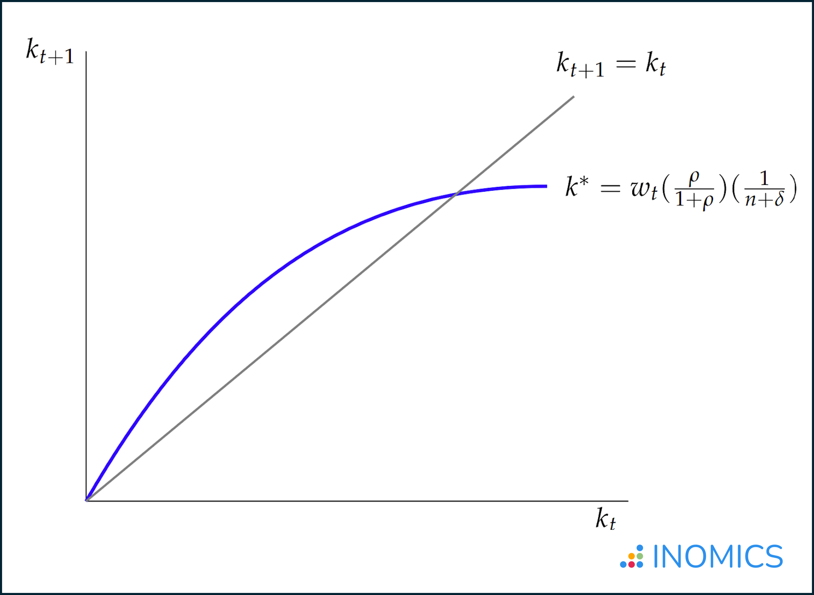
^{Figure 1: The basic OLG model}

Dynamic inefficiency and fiscal policy

From our earlier discussion about savings, recall that:

• If 𝜌 = (1+r_t) for all agents, the economy will reach a dynamically efficient equilibrium.
• If 𝜌 < (1+r_t), agents are too impatient and save too little. This means that equilibrium could be improved by encouraging more saving by younger agents, which would allow the economy to grow more, leading to more consumption for everyone in the long run.
• If 𝜌 > (1+r_t), the agents are too patient and save too much, depressing current consumption and needlessly reducing overall utility.

When the economy is in a dynamically inefficient equilibrium, the government can use fiscal policy to take action and nudge it into a better growth path where future equilibria result in a higher level of utility. In other words, 𝜌 is a parameter that the government can influence, by making savings more or less attractive – and this in turn affects k*.

In the case where agents are too impatient (𝜌 is too low), k* is too low because there’s not enough savings to grow the economy as much as it could be growing. Therefore, effective fiscal policies could raise the interest rate and encourage more savings to increase k* and reach a strictly better equilibrium. This would be an example of expansionary fiscal policy.

Conversely, if agents are too patient (𝜌 is too high), the economy suffers because there’s too much saving and not enough consumption. Because of diminishing returns, at a certain point each dollar of savings is fueling less future output than the consumption that the money could have been used for instead. In this case, fiscal policies that lower the interest rate may prove useful, i.e. to disincentivize savings. This would be an example of contractionary fiscal policy.

Clearly, fiscal policies can change the incentives around saving, which is one lever by which fiscal policy affects the economy. Other means by which fiscal policies can affect the economy include through taxes, redistribution effects, changing labor participation rates, and more. These other levers will impact k* by influencing the levels of aggregate supply and demand, changing how agents and firms behave, and more. See the linked article on fiscal policy for a more complete discussion of these topics.

One of the most common use cases for the OLG model is examining how social security plans work. The model is often used to predict how policy changes in this area will affect the economy. Let’s turn to this as a further example of how fiscal policy can affect the economy in the OLG model.

Social security in OLG

To see how OLG might be used to examine social security specifically, let’s make some extreme assumptions. Suppose depreciation 𝛿 = 1, such that in every period all new capital must be created.

In our discussion so far, we haven’t defined what agents’ savings actually are. In the standard OLG model, savings allow young agents to save some of their capital for the period when they’re old. Then, in their old period, they supply no labor but instead rent this capital out to firms. Therefore, the return to savings rt is the same as the rental rate of capital rt. Eagle-eyed readers may have noticed this already, since it was always the case in our prior derivations.

This means that, when 𝛿 = 1, the return to savings is zero because no capital can be saved for a later period. This in turn means that there are no savings in the economy at all. Therefore, the old generation has no capital to rent out, thus have no income at all, and starve to death. The economy only grows via population growth and each young generation’s labor.

Obviously, this is rather horrific. But there’s good news: utility could be improved in this extreme scenario by imposing a social security system, specifically by taxing the young to support the old.

Recall that (again using our logarithmic utility function) utility is defined by U = ln(c_Y) + 𝜌ln(c_O), and that the optimal consumption mix we found was c_O = c_Y*𝜌(1+r_t). We can see that consumption in the second period would increase the agent’s utility, though at some rate affected by their level of impatience 𝜌.

The social security system would prevent agents from starving in the second period with a small sacrifice to their consumption in the first period. Due to the logarithmic utility function (which guarantees diminishing marginal returns to the utility provided by consumption), under this system of taxation and redistribution, agents would gain more utility in the second period than they lose in the first. The only case where this would be untrue is the case where an agent is totally and completely impatient such that 𝜌 = 0.

Another way to see this clearly is that, due to population growth, everyone can get back more than they put into the system. Recall that L_t+1 = (1 + n)L_t. Since the economy grows at rate n, there are n more individuals in each successive generation that must give some income to only L_t-1 = (1/(1 + n))L_t individuals (n is positive, which means (1/(1 + n)) is less than 1).

In other words: since each successive generation is larger, the amount of money taken from each young agent is less than the amount of money that each old agent receives. Thus, each agent receives a greater social security payment in their second period than they paid in their first period.

However, if we remove the assumption that the population is growing, it may be that L_t-1 is actually larger than (1/(1 + n))L_t, meaning agents put in more money than the generation before them had to! This is a problem in many advanced economies today, where population growth has not been sufficient to outpace prior generations. The OLG model could be used to help these countries understand the amount of financial burden that may be placed on the younger generation, as well as perhaps the effects of other fiscal policies on the pension system with a declining population.

Further Reading

The US Congressional Budget Office (CBO) uses the OLG model to help determine the future effects of fiscal policy choices. Although it mostly refers to the specific model as a “life-cycle growth model”, on slide 1 of the CBO’s “An Overview of CBO’s Life-Cycle Growth Model”1, it states clearly that “The life-cycle growth model (also called an overlapping-generations, or OLG, model) is one model that CBO uses to estimate the long-term effects of changes in fiscal policy.”

Although their version of the model is more complicated than the one we’ve examined in this article, it’s nevertheless built on the same foundation. It’s both instructive and very interesting to read the details of the model that they’ve built, and how the model solves for the predicted state of the economy. You can check out the specifics of their OLG model by reading the CBO’s document yourself!