The Solow-Swan model is an economic growth model that uses a production function (often Cobb-Douglas) to determine the long-term growth path of an economy. It further shows how the economy trends towards a steady state level of capital per capita, depending on the savings rate, and allows us to determine what the best possible savings rate would be.

This cornerstone growth model is often taught in introductory macroeconomics courses, re-taught in-depth for advanced courses, and used as the basis of many other models of the economy, so it helps to get familiar with it.

The Logic Underpinning the Basic Solow-Swan Model

The logic underlying the model is straightforward. In the Solow-Swan economy, individuals have savings rates that yield an economy-wide average level of saving, s. Money not saved in each period is consumed. Meanwhile, savings are used to fuel investment I that grows the capital stock. There is a natural depreciation of the capital stock, denoted by ẟ, over time. For the purposes of the model, there is no foreign economy to trade with, so the Solow-Swan economy is a closed economy (or “in autarky”). With the model, it’s possible to assume the population and level of technology are growing, and possible to assume they are not. These facts come together to determine economic growth, Y. The exact specifics of this relationship depend on the functional form of the specific production function chosen. 

Generally, the more savings an economy has, the more capital stock and therefore economic output it can support. However, with more capital stock comes more depreciation. In per capita terms, there is a limit to how much growth the economy can sustain given its savings rate. 

The model predicts that the economy will trend towards a “steady-state” where the savings rate and the rate of depreciation offset one another such that the per capita amount of capital remains unchanged. In other words, while the overall economy can be growing in size, the population, depreciation, and (per capita) capital stock grow alongside it such that all individuals have a consistent amount of income in perpetuity.

Figure 1 shows the basic Solow-Swan model graphically.

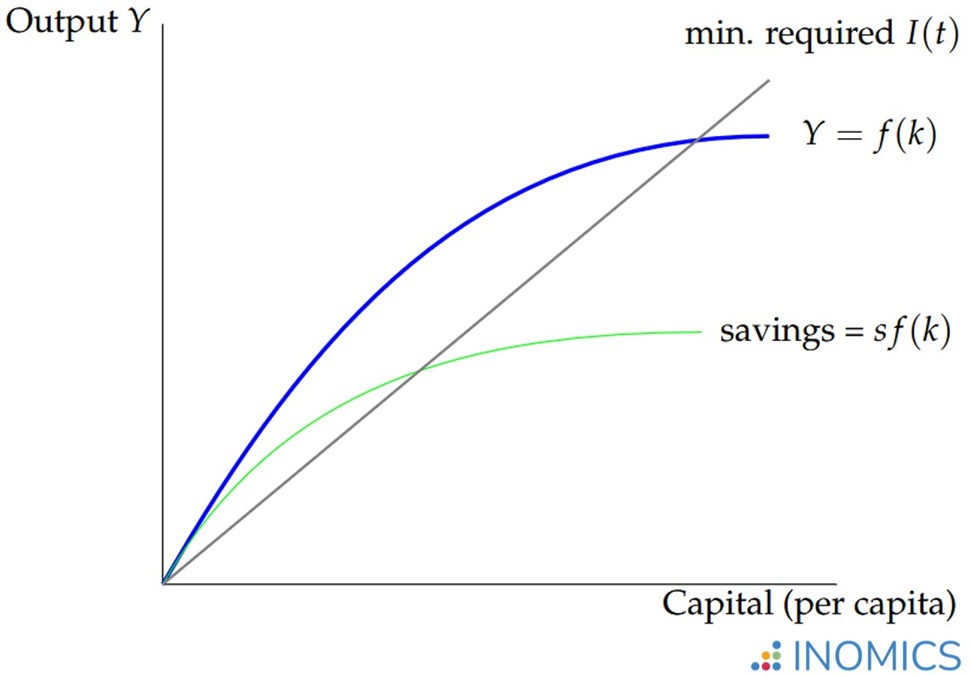
Figure 1: the Solow-Swan model

This graph depicts the general train of logic discussed above. The economy produces goods (here, capital k) according to a production function. This production grants individuals their income. Some part of people’s income is saved, and overall savings are depicted by the green curve sf(k).

Depreciation and the “law of motion” (defined below) are hinted at by the “minimum I(t)” line. This line shows how much investment the economy needs in order to prevent the total capital stock from diminishing due to depreciation. 

Since investment is fueled by savings, the economy must choose an amount of savings that is above or equal to the minimum investment line. Otherwise, the economy shrinks in the next period as depreciation outpaces production.

The next sections dive into the mathematical formulation of the Solow-Swan model, which is critically important – and frequently tested in economics courses. It will describe in math symbols what the above discussed in words, then dive deeper into the model’s behavior.

The Math Behind Solow-Swan

To start building the model mathematically, some core assumptions must be made:

• Time is discrete (e.g., = 1, 2,..., but t ≠ 1.5) and continues infinitely.
• The economy is composed of households that are identical. Importantly, this means all households have the same savings rate s. We assume this is a constant.
• Assume that every person in the economy is a worker and makes up a part of the total labor force L.
• The economy is also composed of individual firms that compete in competitive markets and take all prices as given. Because of this, prices can be normalized to 1.
• The economy produces only one good, which is the capital used in production. This is sufficient for the economy to function normally.
• There are constant returns to scale.
• There are positive and diminishing marginal returns to the factors of production.
• There is no growth in either the population or the level of technology.

Many of these assumptions can be removed, and advanced courses will explore the implications of removing them.

First we need to represent competitive, optimized firms, which are actors in the economy (together with individuals). In both the Solow-Swan model, as in real life, firms can solve an optimization problem.. depending on the functional form of the production function. This is:

max._L≥0,K≥0 Y = (1)F(K,L,A) - wL - rK

where Y is output, F(K,L,A) is the production function F (for example, this could be Cobb-Douglas) with factors K, L, and A (representing capital, labor, and technology), w is the wage rate paid to labor L, and r is the interest rate of capital K (this can also be thought of as a rental rate, as if firms “rent” the capital from households). The term “(1)” represents the price of the final output, which we assume firms can’t choose (since they’re perfectly competitive) and which is therefore normalized to 1.

Note that the term “maxL≥0,K≥0”shows this is a maximization problem where choices of both labor and capital cannot be negative. Firms solve this optimization problem by taking the partial derivative with respect to L and K, the two factors they must utilize. This shows that firms employ labor and capital up to the point where the marginal productivity of each is equal to their cost:

𝝏FL(K,L,A) = w

𝝏FK(K,L,A) = r

As a side note, keep in mind that since a functional form for the production function was not defined, we cannot find the exact form of the partial derivatives above. Often, economics classes won’t choose a production function (because it isn’t necessary when discussing theory), instead referring to some unknown production function F(K,L,A). If we decided to use a basic Cobb-Douglas function, these first-order conditions would become:

𝝏FL(K,L,A) = 𝛼AL𝛼-1K𝛽= w

𝝏FK(K,L,A) = 𝛽AL𝛼K𝛽-1= r

Since firms employ labor and capital up to the point where the cost of utilizing them is equal to their marginal productivity, and since prices are set by the competitive market and not by firms, this means that firms are making zero profits in equilibrium – in other words, this economy exhibits perfect competition. Therefore, when studying the Solow-Swan model, we can ignore the question of who owns which firms.

Mathematically Reaching the Steady-State Equilibrium

Above, we defined how individual firms behave in this economy. Now, it’s time to find out how firms’ output causes the economy to grow over time in the Solow-Swan model. This requires defining several equations that state many of the same ideas we reached logically before. In the following, (t) denotes time.

First, Y(t) = C(t) + I(t), since income (Y) is either spent (C, which stands for consumption) or saved (which is equivalent to investment I by the savings-investment identity). Since the economy is closed, there is no foreign trade (net exports NX = 0), and we assume there is no government spending (G = 0). Combining this fact with the equation we just defined yields:

I(t) = S(t)  = Y(t) - C(t)

Where S(t) is savings across the economy. We assumed that individual households save a constant fraction s of their income Y, which means that the above can be transformed again and then rearranged to yield:

S(t) = sY(t) = Y(t) - C(t); rearranging,

C(t) = Y(t) - sY(t) or, equivalently C(t) = (1 - s)Y(t)

This shows that consumption is a function of income minus savings.

Next, we examine the growth of the capital stock. Logically, the amount of capital K in the next period is equal to the amount of capital the economy has now, minus capital that depreciates during this time period, plus new capital made in this period (as a result of investment I(t)). Putting this logic into math terms, we get:

K(t+1) = K(t) - ẟK(t) + I(t), which simplifies to K(t+1) = (1 - ẟ)K(t) + I(t)

where ẟ represents depreciation (capital that is worn out and ruined from being used). 

We can replace I(t) in this equation to show how the Solow model achieves its steady-state equilibrium. Our next step is to recognize that I(t) = S(t) = sY(t) as above, and replace it in this equation:

K(t+1) = (1 - ẟ)K(t) + I(t) = (1 - ẟ)K(t) + sY(t)

Rearranging, and replacing Y(t) with the (unknown) production function:

K(t+1) = sF(K,L,A) + (1 - ẟ)K(t)

This last equation describes the Solow-Swan model’s equilibrium state! It shows that the evolution of capital stock in the economy is a function of the savings rate plus the amount of capital left over from each previous period. This is known as the “law of motion” in the Solow-Swan model.

Interpreting The Steady-State Equilibrium

This isn’t just an ordinary static equilibrium. Since the model defines growth over time, the law of motion describes the economy’s equilibrium growth trajectory over the entire course of the future.

As we stated before, in the long run the economy grows such that each successive generation of people has the same income in per capita terms as the previous generations, even though the economy is growing in absolute terms. To examine the model further, we transform these equations into their per capita equivalents.

To do this, we divide each variable by the population, which in our case is labor L (because we assumed that all households are composed of workers). Economists denote these per capita variables with a lowercase letter. 

For example, we divide the evolution of capital stock K(t+1) by L to yield (K(t+1))/L, and redefine this as simply k(t+1). Economists will also divide the general form of the production function by labor to yield F(K/L,L/L,A/L) = f(k,1,A/L). When we apply this method to the entire law of motion equation, it yields:

k(t+1) = sf(k,1,A/L) + (1 - ẟ)k(t)

This may seem silly or redundant since we’ve just changed some letters to lowercase and divided everything by the same factor. But, this step helps economists to state clearly in mathematical terms what’s happening – we’ve shifted our analysis from looking at economy-wide statistics to simply looking at each person’s slice of the total economic pie. This helps to reveal an important truth about the model, because in the Solow-Swan model, the growth of the total economic pie can be very different than growth in individuals’ well-being.

Now that the model is in per capita terms, we can define the steady-state level of capital stock per capita that solves the law of motion equation as k*. This is the point where each subsequent year’s per capita capital stock is the same as the year before it – the amount of capital stock (and therefore income) dedicated to each individual is unchanging. Or, in mathematical terms, k* solves the following equation:

k* = sf(k*,1,A/L) + (1 - ẟ)k*

At the steady state, while the overall amounts of capital, labor and output can be changing, the per capita amounts are not! Inserting a production function and solving for k* yields: 

k* = s / ẟ

This relation shows that the steady-state level of capital is equal to the ratio of savings to depreciation. In other words, it shows that the relative size of the savings rate compared to the depreciation rate determines how much k the economy can support in perpetuity.

If we allow for population and technology growth in the model, the law of motion becomes:

k(t+1) = sf(k,1,A/L) - (n + g + ẟ)k(t)

And the solution in terms of k* becomes:

k* = s / (n + g + ẟ)

where n is the population growth rate and g is the technology growth rate. In essence, this equation has the same meaning. It additionally accounts for the fact that output must grow along with the population, and must keep pace with technology growth (so that individuals aren’t using outdated equipment).

Graphing and Convergence

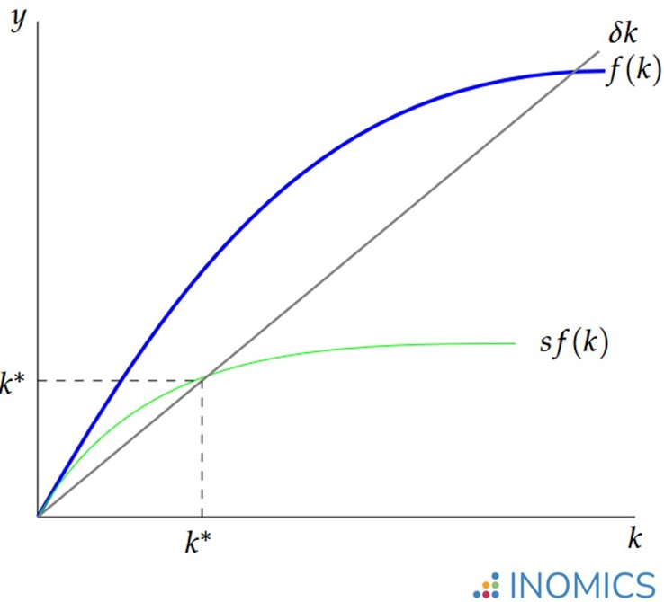
Figure 2: the Solow-Swan Model in per capita terms

Figure 2 shows the Solow-Swan model graphically in per capita terms. The following discussion is in per capita terms as well. In the graph, sf(k) represents the savings rate, f(k) shows overall productivity (and therefore income), and ẟk shows depreciation of the capital stock.

The Solow-Swan model’s law of motion means that the economy trends toward k* over time. The graph helps visualize this truth. Notice how k* appears at the point where the curves for capital production per capita (determined by savings times output, sf(k)), and depreciation ẟk meet.

Given s, if the economy were producing at a point k1 > k*, the graph clearly shows that depreciation would outpace the production of new capital – because where k1 > k*, the line ẟk is greater than the curve sf(k). This means that each subsequent period would have a slight decrease in the amount of capital per capita, until depreciation and the production of new capital balance each other out. This happens precisely where the two lines intersect – at k*.

If the economy produces capital at a point k2 < k*, meanwhile, the economy’s production of capital stock per capita outpaces depreciation – shown where the line ẟk is below the curve sf(k). In this range, the amount of depreciation increases as the amount of capital per capita rises, until the two forces balance each other at k*.

This convergence occurs (mathematically speaking) due to the fact that depreciation increases linearly while production increases with diminishing returns.

But, k* in Figure 2 looks a little small. How can we tell when the economy has reached the best possible steady-state k*?

Savings and the Golden Rule

That question brings us to one last aspect of the Solow-Swan model: how the savings rate s affects the economy, and how to find the best savings rate.

Take a look at how s affects the law of motion:

K(t+1) = (1 - ẟ)K(t) + sY(t)

Clearly, the stock of capital – and therefore economic growth – increases as s increases. Increasing s would increase sY(t) and thus K(t+1) (and the per capita level of savings sf(k)), leading to a higher k*.

But, if individuals save too much, they won’t have enough money left over for consumption! Recall the consumption equation we defined earlier:

C(t) = Y(t) - sY(t) or, equivalently, C(t) = (1 - s)Y(t)

Logically, consumption C(t) decreases as s increases. Therefore, economic agents face the important choice of how much to save so that they can consume enough while still contributing to economic growth for future generations.

Graphically, it’s easy to see that if s increases, the per capita level of capital k* that exists in the steady state will increase, because the function sf(k) will increase. This is shown in Figure 3, where savings increased from s0 to s1:

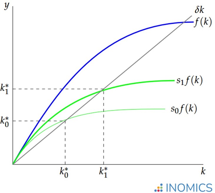
Figure 3: Solow-Swan model after an increase in s

Still, if s increases too much, current generations will suffer as their consumption plummets. The Golden Rule, then, is the rate of savings that maximizes the steady-state level of consumption per capita k* for all generations. It’s called the “Golden Rule” because each generation does to others what they would have wanted done to themselves – they save enough to make sure everyone else can consume the optimal amount in perpetuity.

Mathematically, this can be found by maximizing the per capita consumption equation with respect to k:

maxkc(t) = y(t) - sy(t)

Because we want to solve in terms of k, we manipulate this into an equivalent expression. We know that sy(t) = ẟk in the steady state, and per capita output y(t) is equal to f(k), so we can transform the equation as follows:

maxk c(t) = f(k) - ẟk

Taking the derivative with respect to k, setting equal to 0, and solving then yields:

f’(k) = ẟ

 The amount of k that solves this first order condition is referred to as k*gold. Keep in mind that the specific form of the derivative f’(k) depends on the chosen production function. Astute readers will notice that f’(k) is the marginal productivity of capital, so this finding is equivalent to stating that MPK = ẟ.

It’s easy to “eyeball” this point on the graph. Consumption is equal to the vertical difference between f(k) and ẟk in the graph (because savings is the area under the curve sf(k), and consumption is what’s left of income f(k) after subtracting savings). k*gold is the k* that maximizes consumption – or in other words, it’s where this vertical difference is largest.

The Solow-Swan Model and South Korea’s “Miracle” Growth

The Solow-Swan model can be used to describe growth in many cases in history. For example, it’s well-known that South Korea was a poor nation before the 1960s, and later experienced rapid growth and development that made it one of the world’s most developed nations. This is often referred to as a “growth miracle”.

One of the main reasons for the transformation is that South Korea’s government began to focus on “export-driven industrialization” in the early 1960s. At this time, the government encouraged investment into export industries to increase trade with foreign nations, and also invested heavily into education to develop a skilled workforce. This raised per capita income, which rapidly led to further innovation and industrialization that fueled growth. Today, South Korea has one of the largest GDPs in the world, in both nominal and PPP-adjusted terms.

We can explain this growth using the Solow-Swan model. Before the 1960s when per capita income was near subsistence level, there was very little saving – perhaps putting the South Korean economy on a savings and growth path just like s0f(k) in Figure 3. Once government policies spurred industrialization and invested in education, both per capita productivity and savings grew. 

This would have increased South Korea’s k* as savings increased (just like the shift from s0f(k) to s1f(k) in Figure 3). But there’s more – it would also have caused f(k) to increase, which would cause the optimal balanced growth path k* that the economy could sustain to be greater than before.

Whew! The Solow-Swan model contains an incredible depth of nuance – and advanced courses will dive much deeper. Still, if you’ve made it this far, congratulate yourself with a well-earned break!