A Cobb-Douglas production function models the relationship between production output and production inputs (factors). It is used to calculate ratios of inputs to one another for efficient production, and to estimate technological change in production methods.

The general form of a Cobb-Douglas production function for a set of \(n\) inputs is

\[Y=f\left(x_{1},x_{2},...,x_{n}\right)=\gamma\prod^{n}_{i=1}x^{\alpha_{i}}_{i}\]

In this formula \(Y\) stands for output, and \(x_{i}\) for input \(i\). Meanwhile \(\gamma\) and \(\alpha_{i}\) are parameters determining the overall efficiency of production and how output responds to changes in the input quantities.

The application of this functional form in measuring production is owed to the mathematician Charles Cobb and the economist Paul Douglas. They used it to consider the relative importance of the two input factors, labor and capital, in manufacturing output in the USA from 1899 to 1922.

In their original model, Cobb and Douglas restrict the output-elasticity parameters \(\alpha_{1}\) and \(\alpha_{2}\) to the range \(\alpha_{i}\in\left(0,1\right)\) and to sum to one, which implies constant returns to scale.

The function is thus

\[Y=\gamma x^{\alpha_{1}}_{1}x^{1-\alpha_{1}}_{2}\]

where \(x_{1}\) and \(x_{2}\) stand for labour and capital, respectively. Another common representation of this formula that macroeconomics students may see is:

\begin{equation*}\mathit{Y} = \mathit{A}\mathit{L}^{\alpha}\mathit{K}^{\beta}\end{equation*}

Taking the natural logarithm of both sides of the first equation yields

\[\ln{Y}=\ln{\gamma}+\alpha_{1}\ln{x_{1}}+\left(1-\alpha_{1}\right)\ln{x_{2}}\]

such that for data on output, labor and capital, the parameters \(\gamma\) and \(\alpha_{1}\) can be estimated using Ordinary Least Squares.

Based on their data, Cobb and Douglas find a value of 0.75 for \(\alpha_{1}\). This implies that labor accounted for three quarters of the value of US manufacturing output (capital accounting for the remaining quarter) over the period studied.

Their estimate for the efficiency parameter \(\gamma\) is 1.01. Since it is greater than 1, this reflects the positive effects of unobservable forces on production through the combination of labour and capital.

The multiplicative nature of a Cobb-Douglas production function, assuming positive values for \(\alpha_{i}\), means that the inputs are complements in production. In the standard model of labor and capital, increasing the amount of capital increases production both directly and indirectly through its impact on the productivity of labor.

Mathematically, the cross-partial derivative of production output \(Y\) with respect to labor \(x_{1}\) and capital \(x_{2}\) is positive.

Furthermore, due to the assumption that \(\alpha_{i}\in\left(0,1\right)\), the second-order partial derivatives of production output with respect to labor and with respect to capital are both negative. This suggests diminishing marginal returns for each input alone. Simply adding either more labor or more capital (but not both) to the production process increases output, though at a diminishing rate.

Additionally, the elasticity of substitution between the inputs is constant and equal to one due to the functional form. A two-input Cobb-Douglas production function can be represented graphically in the form of isoquants: combinations of both inputs for which the output is constant.

There are four such isoquants in the graph here for the (constant) output levels \(\overline{Y_{1}}\), \(\overline{Y_{2}}\), \(\overline{Y_{3}}\) and \(\overline{Y_{4}}\). The further the isoquant from the origin, the greater the level of output \(\overline{Y_{4}}>\overline{Y_{3}}>\overline{Y_{2}}>\overline{Y_{1}}\).

Which precise combination of the inputs \(x_{1}\) and \(x_{2}\) is optimal for production is determined by the budget available to the producer as well as the cost ratio of input \(x_{2}\) to input \(x_{1}\). These factors can be included in the graph in the form of an isocost line (see the article on elasticity of substitution).

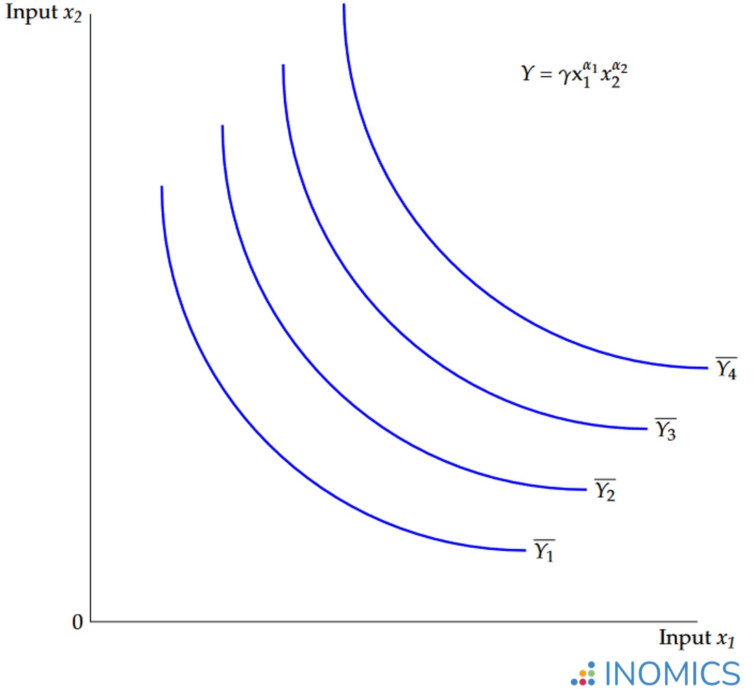
Figure 1: Cobb-Douglas production function isoquants

Cobb and Douglas themselves acknowledged that their production function does not rest on solid theoretical foundations, nor should it be understood as a law of production. It merely represents a statistical approximation of the observed relationships between production inputs and output. Nevertheless, its simple mathematical properties are attractive to economists and have led to it becoming a standard in microeconomic theory over the past century.

Further reading:

For the background and an overview of the main properties of Cobb-Douglas production functions, see in particular sections 6, 7 and 8 of Cobb and Douglas’ original article, “A Theory of Production” (The American Economic Review, 1928).

Good to know:

The Cobb-Douglas functional form is not only used in the theory of production but it has also become standard in microeconomic consumer theory. There it is applied as a utility function, where \(Y\) becomes \(U\) for utility. The \(x_{i}\) then represent items of consumption. When the utility function is maximized, subject to a budget constraint, the values for \(\alpha_{i}\) indicate how the individual will optimally distribute their budget among items.