Utility in economics refers to the level of happiness or satisfaction of individuals. Individuals derive utility from the consumption of goods and services, and seek to maximize their utility under any given budget.

The assumption that individuals maximize utility is a cornerstone of microeconomics. It is used as a basis to explain market behavior and to predict how people act and react in particular situations. Individuals are assumed to be perfectly rational, capable of calculating how much utility they will obtain from any combination of goods and services, and choosing a combination where utility is maximized, subject to their budget constraint.

In most economic modeling, an individual’s utility is described as a continuous, monotonic, and concave function of consumption. That is, the utility function U(X), where U stands for utility and X for consumption (X can be a vector of goods and services consumed), is continuous over the space of X. Its first derivative with respect to X is positive (“more is better”) and its second derivative with respect to X negative, representing the law of diminishing marginal utility. 

The individual will, in most cases, be limited in consumption by their income such that spending on goods and services X cannot exceed a maximum level M. The individual’s maximization problem can be posed as

\begin{gather*} \max_{X}U\left(X\right)\\ \text{s.t.: }XP\leq M \end{gather*}

where P is the corresponding vector of prices for the goods and services X.

Figure 1 depicts a simple two-dimensional case where the individual chooses between combinations of items X₁ and X₂ (item X₂ might also represent “all other items” in order to study the individual’s choices of X₁ compared to alternatives).

The items’ prices P₁ and P₂ and the budget M determine the set of choices the individual can make. They could devote their entire budget to X₁, purchasing Q_X1 at a cost of P₁Q_X1 = M, or they could do the same for X₂, purchasing Q_X2 at a cost of P₂Q_X2 = M. All affordable combinations of X₁ and X₂ are found in the grey shaded triangle which is limited by the budget line P₁X₁ + P₂X₂ = M running between the points (Q_X1,0) and (0,Q_X2). 

A set of indifference curves is drawn in the graph as well. Indifference curves are defined as combinations of X₁ and X₂ that give the individual a fixed level of utility (hence the individual is indifferent between such combinations). Due to utility increasing in X, indifference curves further from the origin (0,0) represent higher levels of utility. 

The individual’s utility is hence maximized at the point where the budget line is tangential to the “highest” indifference curve IC at the point (q_X1,q_X2), resulting in utility Ū. This means that the person will choose to buy q_X1 units of X₁ and q_X2 units of X₂; this mix is the optimal choice. On the indifference curve IC’ the individual would obtain even higher utility U’, however this is not attainable given the individual’s current budget M.

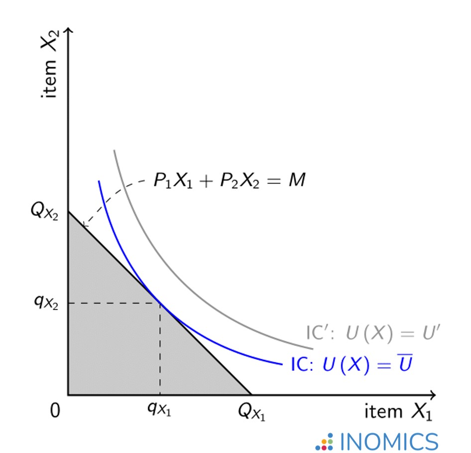
Figure 1: A budget constraint with standard indifference curves

Non-economists may balk at the idea that individuals calculate budget lines and indifference curves in order to make their consumption decisions. This need not be the case for the theory still to have traction. It is sufficient for the economist if individuals act as though they were maximizing utility. 

Utility maximization need not be a conscious or explicit process. What is important for an economist is to be able to observe behavior and then explain what is observed. Decisions that are consistent with utility maximization allow individual preferences to be summarized through utility functions, which is convenient for the analyst. Economists tend to value observing what people do (“revealed preference”) more highly than simply recording what they say they do or will do (“claimed preference”).

Insofar as the future state of the world is uncertain and decisions are made under uncertainty, individuals can be assumed to maximize expected utility. This is the utility to be gained from each possible state of the world, weighted by the probabilities of the various states of the world being realized. 

A utility function can also be used to describe the individual’s attitude toward risk. For example, a risk-averse individual will tend to prefer lower but more certain levels of consumption over potentially high but very uncertain levels of consumption. In this case, the utility function will be strictly concave.

Solving the utility maximization problem

There are two main methods for solving a utility maximization problem, which students of microeconomics will become very familiar with. The first is the graphical method, explained below. The second is the Lagrange method, which is explained in the linked article.

To solve utility maximization using the graphical method, it’s helpful to start with some logic. We already know that the best indifference curve is the one that is the highest attainable curve given the budget constraint. In Figure 1, this is shown as the point (q_X1,q_X2). At this point, the budget line is tangent to the indifference curve.

Why is this? If the indifference curve is too far to the left, it is an affordable but undesirable product mix. The consumer could benefit by consuming a bundle of goods on indifference curve IC instead. Meanwhile, it’s already been established that indifference curve IC’ is not feasible because it’s too expensive for the consumer. So, any indifference curve that is best must be tangent to the budget line, like the curve IC. A curve that is tangent will be as high as possible (as it only touches the budget line at one point), and guarantees that the individual must use their entire budget to reach it.

This fact allows us to construct an equation that we can solve. Because we know that the best indifference curve is tangent to the budget line at the point (q_X1,q_X2), we know that both must have the same slope at this point. So, all we need to do is set the slope of the budget line equal to the slope of the best indifference curve and solve.

The slope of the budget line is simply the price ratio between goods X₁ and X₂, or how much more of X₂ the individual could buy if they gave up one unit of X₁. Recall from algebra that the slope of a line graphically is the “rise” over the “run”, or in this case, P₁ / P₂. Also note that the budget line is downward-sloping; this is because to afford more units of one good, some of the other must be given up.

The slope of the indifference curve is equal to the ratio of marginal utility between the two goods, also known as the marginal rate of substitution. This is because the curve measures how much of X₂ the individual would be willing to give up to have one more unit of X₁ and still be at the same level of happiness or utility (hence the term “indifference”).

If we set the price ratio (the slope of the budget line) equal to the ratio of marginal utilities for this individual (the slope of the indifference curve), we can solve for the utility-maximizing point.

Setting these equal to each other yields the following equation:

\begin{equation*}
        \frac{\mathit{P}_{1}}{\mathit{P}_{2}} = \frac{\mathit{MU}_{1}\left(\mathit{x^*_1},\mathit{x^*_2}\right)}{\mathit{MU}_{2}\left(\mathit{x^*_1},\mathit{x^*_2}\right)}
    \end{equation*}

This equation can be solved by plugging in the prices of each good on the left-hand side, inserting the marginal utility on the right-hand side, and solving. This yields the optimal product mix, which can then be re-inserted into the budget constraint to find the individual’s utility-maximizing consumption decision.

Remember that the marginal utility is the first derivative of the utility function, so MU₁(x*₁,x*₂) is the first derivative of U(X) with respect to X₁. See the exercise to practice this concept.

The Lagrangian method is another, very common method used by microeconomists to solve constrained optimization problems. Check out our linked article to learn this method as well.

Further reading

Two economics Nobel laureates, Daniel Kahneman (2002) and Richard Thaler (2017) are both known for criticizing the assumption of individual rationality in economic theory and for offering plausible alternative behavioral insights. See their joint paper, “Anomalies: Utility maximization and experienced utility” (Journal of Economic Perspectives, 2006) for an excellent discussion of the limited human capacity to reason about personal well-being, in particular when time passes between consumption decisions and consumption itself.

Good to know

While modern behavioral economics throws individual rationality and the idea that people always maximize utility into doubt, the theory of utility maximization can also be applied to decision-making in organizations, where one might reasonably expect choices to be made with more calculation and deliberation. The theory is also widely applied in welfare economics where government decisions are justified based on the idea of maximizing a social-welfare function, which is basically an aggregate representation of people’s preferences in society.

Practice solving a utility maximization problem

Exercises for you