Regression is a word commonly used in econometrics, statistics, and many other sciences. It describes a widespread technique used by scientists of all kinds to empirically test theories using available data.

The name is attributed to Sir Francis Galton, who lived in the late 19th century and coined the term while studying people’s heights. In his study, Galton collected the height measurements of parents and their children.

He noticed that particularly tall parents tended to have children who were tall, but somewhat less so than their parents; meanwhile, short parents had children who were short, but still taller than they were. From these data points, Galton surmised that the heights of children tended to “regress” back towards the average adult height, rather than perfectly continue the height trend of their parents.

Despite this word not really reflecting the actual statistical process of analyzing the variance of height data, it stuck. We use the word “regression” to describe a wide variety of models and analyses used by scientists – including economists – today.

The basics of regression

A regression is a method of analysis where an economist (or other scientist) uses data to measure the amount of variation in their topic of interest that is explained by various factors. This is often used as evidence to show that these factors affect the topic of interest, and how they do so. The most intuitive type of regression is a simple linear regression, explained as follows.

The main subject the economist is interested in is (usually) the dependent, or y, variable (sometimes also called the response variable). This variable is something the economist wants to learn more about; for example, y could be test scores for students in a class. The various factors used to explain the variation in y – in our case, test scores – are the independent or x variables. These can be anything that might reasonably affect test scores, such as nutrition, IQ, age, hours spent studying, the parents’ level of education, and more.

The economist then collects data on each of the variables. With the data, the economist constructs a matrix or table and uses their method of choice for calculating the amount of variation in y that the x variables explain. This is done by mathematically comparing how much y and a given x variable vary “together” or “at the same time” – in other words, how they co-vary. The economist takes this to mean that x can explain a certain amount of the variation in y, and probably has a meaningful real-world relationship with y.

An easy way to get started is to view the data in a scatterplot to see if there appears to be a relationship. Figure 1 shows that there is an imperfect but probable linear relationship between y and x.

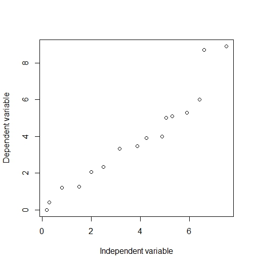
Figure 1: A scatterplot of y and x made using R.

This can be a good starting point to suggest, like Sir Galton, that there is a real phenomenon at work. In order to study this more intensely, an economist will go on to define an equation and do some math.

A simple linear regression equation

The regression is described by an equation. In the simple linear case, this is as follows:

\begin{equation*}
        \mathit{y} = \beta_0+\beta(\mathit{x})+\epsilon
    \end{equation*}

where y is the dependent variable and x is the independent variable that the economist believes influences y through an economically meaningful relationship, as described above.

\(\beta_0\) is a Greek letter that will be a number once the equation is calculated, and is the y-intercept of the equation. \(\beta\) similarly stands for the numeric coefficient on x in this linear equation. Normally, the economist checks to see whether the \(\beta\) coefficient(s) on x are “statistically significant”. Those that are show evidence that they affect y in a non-random way.

These numbers represented by \(\beta\) are calculated as a result of whichever statistical method the economist chooses to use for this equation. Recall our earlier example, where y is the student’s test score and a possible x variable is the student’s hours spent studying. Let’s suppose that calculating this regression equation results in the following:

\begin{equation*}
        \mathit{y} = 25.00+15.67\mathit{x}+\epsilon
    \end{equation*}

This equation can be interpreted as follows: if the student spends no time studying, x = 0 and the equation simplifies to y = 25.00 (plus \(\epsilon\), but this is expected to be zero; more on \(\epsilon\) later). This means a student who does not study at all is expected to score a 25 on the exam.

For every 1-unit increase in x, the student is expected to earn 15.67 more points on the exam. This means that every extra hour spent studying is expected to raise the student’s exam score. It seems like studying is a useful activity, then. If a student studies for four hours, they’re expected to earn an 87.68 on the exam.

Although there was only one x variable in this example, it’s important to know that multiple x variables can be used. When this is the case, the regression is known as a “multiple linear regression”.

Finally, \(\epsilon\) is the “error term”. The error term accounts for all of the variation in y that is not explained by x, allowing this equation to hold true. Because of this, it’s often thought of as a variable that captures the effects of all other variables that affect y and aren’t included in the regression.

Residuals are another important term related to \(\epsilon\) – each individual “error” data point is a residual, such that \(\epsilon_i\) is a residual. Residual analysis usually refers to looking at a chart of the residuals, which gives the economist an idea of how well-behaved the error term is – and if any corrections should be investigated for the model in question.

The error term is a very important part of regression analysis. On the one hand, the goal of the regression method is usually to minimize error – as this results in an equation that most closely mimics the behavior of y in the data.

Further, studying the error term for a specific regression model can give the economist evidence that the model is (in)correctly specified, suggest the presence of biases or missing variables in the model, and more. In order to conduct an acceptable econometric analysis, economists often must prove that the error term in their equation behaves as expected. This usually involves showing that the error term has an expectation of zero and can be thought of as random, patternless noise.

Types of regression models

The above example did not mention how to actually generate the numbers in the equation. There are many methods that an economist can use to do this, thereby calculating the regression. Normally, economists use software to quickly calculate their regression equations, but it’s possible to do many regressions by hand.

In fact, many economics students will be taught to generate a regression in class using the common and foundational Ordinary Least Squares (OLS) method for a linear regression analysis. This method calculates the regression coefficients and the error term using the “sum of least squares”, which is a simple and surprisingly powerful way to find the regression equation that minimizes error.

Other models commonly used in economics besides OLS include (Feasible) Generalized Least Squares (FGLS), probit and logit, Maximum Likelihood estimation (MLE), Ridge and Lasso regression, and polynomial regression. Econometrics can also blend into machine learning and data science, sometimes utilizing regression models like Decision Tree and Random Forest, depending on the goal of the analysis.

Goodness-of-fit measures

An economist can set up a regression equation for just about anything. For example, we could have used not just hours spent studying, but age, IQ, and parent’s education level in our linear regression model example above. In fact, nothing stops us from making multiple regressions with every combination of these variables to try and predict y. How does the economist decide what the best model to use is?

The first step is that the economist should derive an equation from theory first. Whatever relationship the economist expects is true in reality is a very good starting point.

There are numbers generated from statistical concepts called goodness-of-fit measures that can help economists understand which model generates the best fit for the data. The most commonly used measure, R², is typically used for linear regressions. It describes how much variation in y is explained by the regression equation, on a scale from 0 to 1. Ceteris paribus, an economist would prefer their model to have a higher R² than other models, if y is their main variable of interest and they’re trying to explain variation in it.

However, a promising goodness-of-fit measure alone does not mean the regression is a good one. Every regression needs sound economic reasoning behind it to be considered valid. This idea is explored more fully in the following section.

Limitations of regressions

Once students learn how to run a regression, it’s easy to think that this type of analysis can answer all kinds of questions. And, regressions really do help economists answer many questions about economic theory and the real world. But there are important shortcomings to know about regressions before utilizing them.

First, it’s useful to understand that regression analysis simply analyzes how much y co-varies with each x variable and the model as a whole. Often, students can internalize simple (but incorrect) shorthand, such as “x causes y because the regression results are significant”. While this interpretation might end up being true, regression significance is not sufficient evidence to prove causation. Additional proof is needed.

For that reason, regressions require sound theory behind them in order to convincingly show any economic relationship. It’s easy to design regressions that have amazing statistical qualities, highly significant variables, and large R² values – but are ultimately meaningless. This is often due to a problem known as “spurious correlation”, which means two variables that have nothing to do with each other show a high degree of covariance anyway.

For example, the following humorous chart from former Harvard student Tyler Vigen shows that the number of movies Nicolas Cage appeared in is highly correlated to the number of people who die by drowning:

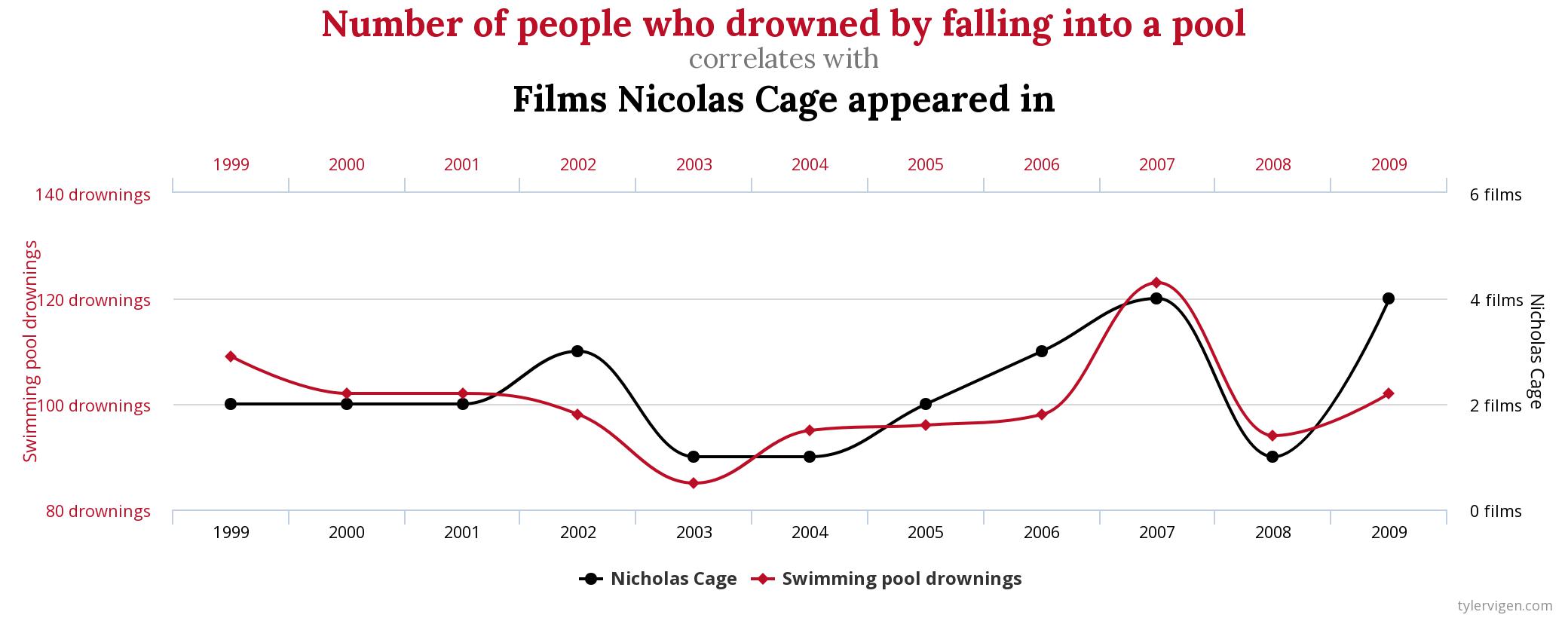
If one were to run a regression of this data, where deaths by drowning were coded as the y variable and Nic Cage movies were the x variable, the results would show a relatively high R² and a significant effect of x on y. In this way, simply looking at the regression results of y on x without considering economic theory, it would be easy and understandable to think that x must be an important cause of y. But clearly, Nicolas Cage appearing in movies has (almost certainly) nothing to do with the risk of people drowning!

Regression analysis is one of the main tools that economists use to conduct research, test economic theory, and learn about the real world. It’s an invaluable skill for students of economics to learn. Those who are very interested in regressions should consider majoring in econometrics, economic statistics, or a similarly quantitative option.

Further Reading

This article has only covered the tip of the iceberg when it comes to regression analysis. And, for the interested student, good news – there are literally thousands of articles and books written on the subject.

Some classic introductory texts that don’t require too much math expertise include Regression Analysis and Linear Models: Concepts, Applications, and Implementation by Darlington and Hayes, and Applied Linear Statistical Models by Neter, Kutner, Nachtsheim, and Li.

Good to Know

Regressions in economics literature are very important. Essentially all serious empirical economics research includes a regression analysis, which is typically presented alongside a lengthy theoretical explanation of the expected relationships at hand.

The best papers include convincing justifications for why the model fits the data, what it means, and discussions of weaknesses and drawbacks to the authors’ approach. Students who are interested in economics research would be well served finding a good empirical economics paper to learn from. Additionally, the following recommendations from the German IZA Institute of Labor Economics and Plamen Nikolov give a detailed and helpful breakdown about what’s expected of an empirical economics paper.