Economists often run into situations where they need to type out mathematical formulae or draw up a graph, especially for research papers. But, anyone who’s attempted to do so knows that math symbols and complicated graphs are very difficult to produce using typical word processor options. So, what’s a humble econometrician to do?

Enter LaTeX, a typesetting system that’s been developed for researchers of all stripes to write and neatly print properly formatted mathematical formulae. If you’re able to learn and use it, you’ll be able to write important documents such as your economics thesis or a research paper in no time.

While LaTeX isn’t the only option economists have to handle this work, it is a commonly used and freely available option. The most common alternatives include Markdown and plug-ins for Adobe InDesign.

That’s right – anyone can get started practicing LaTeX for free, using a popular site called Overleaf. Because the basic version of Overleaf is a free and easy to use LaTeX editor (though paid plans are available for more features and integrations), the rest of this article will assume that the reader is using it.

This is a skill that’s great to have for your economics coursework and future career, and not terribly difficult to learn, so let’s dive into some LaTeX basics.

Before you start: understanding mathematical symbols

The first step to learning LaTeX and writing professional-looking economic formulae is understanding what those formulae are and how they are typically written. We’ve already shared an article that describes many of the commonly used symbols in economics.

If you find yourself struggling to read some of the strange symbols presented in economic formulae during lectures or in textbooks, the linked Math Symbols article is a great place to start. Once you’re familiar with the symbols typically used in economic formulae, continue reading!

Getting started in LaTeX: the preamble

The “preamble” in LaTeX is a section found at the beginning of the document. In Overleaf, this will be at the top of the left-hand side Code Editor section. The preamble is written by the author, and contains important code for setting up the document. This is where you’ll install packages and other functions that you’ll need, as well as set document-wide defaults like margin spacing and font size.

The preamble – and thus the document – always starts with the “\documentclass{}” command. This defines what type of document is being produced. Inside the curly braces can be written a number of words; “article” is probably the most commonly used, and will serve most purposes. Thus, the first line of code is typically “\documentclass{article}”.

Research papers ought to use this command, and it’s also suitable for a casual learner to start using LaTeX. Other document classes tend to be more specialized, such as “beamer” for presentations, “minimal” for debugging and “slides” for a slideshow.

An important fact to know is that you can set certain parameters for your document, and any equation or function that you type, using brackets such as [] right after a command. For example, you can set the font size equal to 12 for your entire document using “\documentclass{article}[12pt]”. We’ll return to the usefulness of these brackets later when we discuss graphing.

Other lines of code that will be entered in the preamble include packages that you’ll need to install, similar to software programs like R that econometricians use. There are many, many packages containing specific and niche tools, and LaTeX does not automatically have access to all of them. So, by inserting lines of code like “\usepackage{pgfplots}”, specific functions will be loaded so that you’re able to access them when you need them.

Some common packages that you may need to install as an economist include, but are not limited to:

• pgfplots: contains useful functions for graphing.
• tikz: another package that contains useful functions for graphing.
• amsmath: developed by the American Mathematical Society (AMS); contains useful functions and improvements for writing equations in LaTeX.
• amssymb: again developed by AMS, contains useful math symbols that you can insert into your document.
• graphicx: allows you to insert images into your document from an external source, like your hard drive.
• tabularx: contains further options when making a table.
• multirow: if you’re using a lot of tables, this package allows entries to cover more than one row, which can be useful.
• mathpazo: sets a standard font used when printing mathematical characters.
• nicefrac: an option for typesetting in-line fractions neatly.
• subfig: allows you to more easily create a figure that’s broken into multiple sub-figures.
• footnote: further options for formatting your footnotes.
• natbib: contains helpful support for handling in-text citations and the bibliography.

If you need more specific packages for your economics coursework, your instructor is likely to provide them for you. If you’re working on your PhD thesis or other research, your supervisor(s) or colleague(s) might be able to help you find specific packages you may need on top of these basic suggestions.

After installing packages, you ought to include lines for the title, author, and date the document was written. The commands for this are “\title”, “\author”, and “\date”; fill these in with braces as with other commands. For instance, if this article was written in LaTeX, it would have these three lines of code:

• “\author{Sean McClung}”
• “\title{A gentle introduction to LaTeX for economists}”
• “\date{October 2 2023}”

At the end of the preamble, you’ll need to write “\begin{document}”. This tells LaTeX that the code below this line is used to actually generate your document.

With the preamble out of the way, you – and this article – are now ready to move on to the meat and potatoes.

Writing your first equation in LaTeX

There are a few commonly used commands that you can use to write an equation in LaTeX. These include (but are not limited to):

• Equation: this will print your equation with a line number, which can be useful in some contexts. Use “equation*” instead if you don’t want line numbers.
• Align: vertically aligns multiple equations (this makes them look neat in your document when printed and avoids awkward spacing). Can also be used to break up multiple equations into columns, should you wish to present them that way.
• Multiline: allows long equations to be split up on multiple lines so that they display properly.
• Gather: Another option to simply print a number of centered equations.

The differences in these options tend to be minor, and in many cases which one you choose won’t affect your output much. But, using the right one for the right niche circumstance can still make the difference between a professional-looking paper and a haphazard one, so it pays to learn the difference.

After you’ve decided on one of the above options (and picked a formula to write!), you’ll be ready to start typing. Simply type out your desired equation using the proper symbols, and LaTeX will be ready to produce professional-looking output of it.

A note – if you need to use fractions, you must do so using the “\frac{}{}” command. This can be confusing at first. However, it’s quite simple to use. The expression in the numerator belongs in the first set of braces, while the denominator goes in the second set of braces. Thus, to type 1/2 as a fraction, you’d enter “\frac{1}{2}”.

Very quickly, you’ll probably realize that you need to insert a specific symbol that isn’t found on a keyboard – like \(\partial\). This is done by first typing a “\” symbol, which tells LaTeX that you’re about to use a special character (or type a new command).

When you do this, a list of symbol and function names will appear next to your cursor. You can scroll this list to choose the option you want, or keep typing to narrow the list. Simply press “Enter” or click on the option you want. You can even type out the entire name and ignore the list, if you wish.

In the coding window, this won’t appear to do much. But, when you compile your work, you’ll see LaTeX print out “\(\partial\)” instead of “\partial” on the document compilation output. Read on for how to compile and check out your work done so far.

The “Recompile” button

You now know how to write formulae in LaTeX. But, since the Code Editor doesn’t automatically show you the exact output, it can be hard to know precisely what you’ve written. Further, at first you’ll probably run into many simple error codes as you get used to the new language of LaTeX. How can you check this to review your progress and make corrections?

At the top-right of your Overleaf screen, you’ll see the “Recompile” button. Clicking this button will execute your LaTeX code. This will cause your entire document to appear as if it was being printed out on the document screen to the right. Then, you can check visually if your formulae turned out as expected.

If there are any errors, the compile will fail, and the document screen will display an error message instead of your work. Helpfully, the offending line(s) on the left-hand side Code Editor will be highlighted with a red symbol. Hovering your mouse over the symbol will show a message describing what went wrong on that line.

Check your code to ensure you’re using the proper syntax, and start small so that it will be easy to identify errors. Search engines like Google are great friends to have during these steps.

Now that you can write equations – and compile the document – here’s an example. Try copying this code in your own Overleaf project, and see if you can manipulate the equation yourself. The following code produces the Cross Elasticity of Demand equation shown below:

• \begin{equation*}
•         \epsilon_{AB} = \frac{\Delta\mathit{q}_{A}}{\Delta\mathit{p}_{B}} = \frac{\frac{{dq}_{A}}{\mathit{q}_{A}}}{\frac{{dp}_{B}}{p_B}}
•     \end{equation*}

\begin{equation*}
        \epsilon_{AB} = \frac{\Delta\mathit{q}_{A}}{\Delta\mathit{p}_{B}} = \frac{\frac{{dq}_{A}}{\mathit{q}_{A}}}{\frac{{dp}_{B}}{p_B}}
    \end{equation*}

Making graphs in LaTeX

Making graphs in LaTeX is intimidating at first, because even a simple graph requires using many different lines of code. However, it’s quite intuitive to create graphs once you get the hang of it. As with writing equations, it’s best to start small. Start with a simple graph as an end goal, and introduce one or two elements at a time until you’ve finished the graph. It will be easier to identify errors and learn that way.

To start drawing a graph using LaTeX, you’ll need to use one of a few commands just like when writing an equation. The most commonly used commands are:

• begin{tikzpicture}: used after installing the tikz package. This line of code tells LaTeX that the following lines are being used to create a graphic of some sort. Then, the line “begin{axis}” should follow for most economics applications.
• begin{axis}: this command will create an x-y axis. You can set its dimensions and scale; it defaults to a maximum x value of 10 and likewise for y values.

The aforementioned brackets are also very useful when creating your axis, allowing you to set the axis parameters. For instance, “\begin{axis}[xmax = 15, ymax = 15]” will create a larger axis than the default, showing elements up to 15 units away from the origin instead of the default 10.

Then, LaTeX expects you to introduce elements via equations or plotting them on the graph, somewhat similarly to how a graphing calculator works. You’ll typically use the “\addplot{}” command to graph equations.

For instance, to add a simple line, you can use a linear equation such as: "\addplot [domain = 1:10, restrict y to domain = 0:10, color = blue, very thick] {x+1}. This will graph the simple line y = x + 1" as a blue line on your graph. A few other useful tricks have been shown in the brackets: you can set the domain as shown, and even restrict the domain of the function if you only want to show part of the line. For example, you can adjust the above command to read “restrict y to domain = 3:5” if you only want to show the parts of y = x + 1 that cross through the points (2,3) and (4,5). You can also produce a dashed line by typing “dashed” instead of “very thick”. Try it!

Of course, lines need labels in economics. You can add a label to your line with the “\node” command, like so: “\node at (4, 1) {$D$}” prints a nice D, for demand curve, at the point (4,1).

Finally, the “draw” command is a useful tool to know about when graphing. It allows you to create more free-form shapes and lines without needing to specify an actual equation to draw them. This can be a great option when you want to draw a graph that involves undefined points, sharp angles, or odd shapes. For example, you can use the command “\draw[dashed,gray] (5, 2) to (5,0)” to draw a dashed, gray line from the point (5, 2) to the point (5,0).

As an example, the following code (with a proper preamble already written) produces the simple graph shown below:

\begin{tikzpicture}
\begin{axis}[
xmin = 0, xmax = 10,
ymin = 0, ymax = 10,
axis lines* = left,
xtick = \empty, ytick = \empty,
clip = false,
scale = 1.5,
]
% Curves
\addplot [domain = 0:10, restrict x to domain = 1:9, color = green, very thick] {-x+10};
\addplot [domain = 0:10, restrict x to domain = 1:9, color = blue, very thick] {x};

\node [] at (9, 0.8) {$D$};
\node [] at (9, 9.2) {$S$};
\node [left] at (0, 5) {$p^*$};
\node [] at (5, -0.3) {$q^*$};
\node [left] at (0, 9.8) {price};
\node [left] at (9.8, -0.3) {quantity};

\draw[dashed] (5,0) -- (5,5);
\draw[dashed] (0,5) -- (5,5);

\end{axis}
\end{tikzpicture}

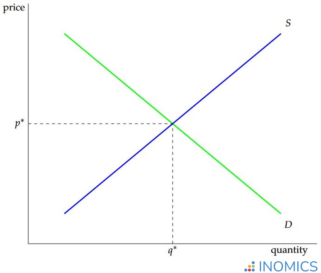
See if you can tell which commands produced which elements on the graph. Try copying this code into your own Overleaf project, and see if you can manipulate the elements. This will help you learn quite swiftly!

Once you’ve started making graphs, and got the hang of it, we have a further practice suggestion for you. All of the graphs in our Economics Terms A-Z were made using LaTeX. Why not pick a graph from one of these articles – such as Demand Curve or Market Equilibrium – and see if you can recreate them in LaTeX? If you’re feeling confident, try making a complicated one like Deadweight Loss or Edgeworth Box.

The “end” command

One final and important note; at the end of each equation, graph, and document, the “end{}” command must be typed with the \ symbol just before it. This is the counterpart to the “begin{}” command that starts a graph, equation, or document. Without a matching “end{}”, you’ll receive error messages.

Fortunately, when you type “begin{}”, this is automatically produced for you in Overleaf. But it still pays to be aware of its importance. If you end up deleting an “end{}” on accident, you’ll receive error messages.

The tip of the iceberg

This article has only shared the very basics of using LaTeX for economics. If you’re just looking to get started with learning LaTeX for practical application purposes, you should now be all set to start writing equations, making graphs, and even drafting your economics thesis or research paper.

But as with most tools and applications, a vast sea of advanced knowledge awaits. If you want to learn more, head over to Overleaf’s “learn” section for more in-depth explanations and tutorials. There are also numerous online resources that will be able to help you find specific code if you’re stuck. Best of luck!

^{Header image credit: Pixabay.}