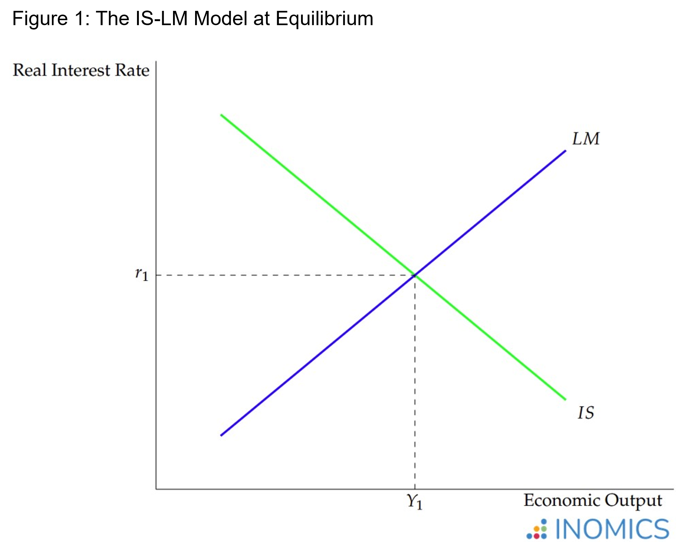
The IS-LM Model is a foundational macroeconomic model of describing the relationship between the interest rate and economic output. Using two curves , it depicts an array of equilibria for the economy and can be used to assess the potential impacts of fiscal and monetary policies.

The two major components of the IS-LM model are the “Investment-Savings” curve (or IS curve), and the “Liquidity preference-Money supply” curve (or LM curve). Where they intersect, the real interest rate and real economic output are balanced, such that the “product market” and the “money market” are in equilibrium; in other words, there is just enough money in circulation to facilitate all of the transactions that economic agents want to conduct.

The model was originally developed in the 1930s by John Hicks, who was expanding on the ideas of John Maynard Keynes. At the time, controlling the money supply was seen as a more important lever for policymakers than it typically is today. Since the IS-LM model can help explain how the money supply influences economic growth (for instance, as measured by GDP), it became a key tool of macroeconomic policy until later that century.

In the 1970s and 1980s, when inflation became more of a major economic concern, the IS-LM model fell out of favor and policymakers started to focus on inflation and interest rates more than the money supply. Despite the model’s limitations, however, economists usually agree that it’s a good foundation for students, and thus it’s still widely taught in introductory macroeconomics courses.

Figure 1 shows the basic IS-LM model in equilibrium.

The IS (Investment Savings) Curve

The graph of the IS Curve shows every point in the economy where overall income and the real interest rate are “in equilibrium”. Thus, the real interest rate r is on the vertical axis and income (or output) Y on the horizontal axis. Yet, these quantities don’t directly affect each other; the curve is effectively hiding equilibrium in two different markets that determine its shape.

These two markets are the “expenditures market” or “Keynesian cross diagram” (the top graph in Figure 2), which shows where income and expenditures in the economy are equal, and the “goods market” (the middle graph in Figure 2), where the real interest rate holds desired savings and desired investment in equilibrium. In a way, the IS curve is built by taking one axis from each of these two diagrams and smashing them together. This is best illustrated with Figure 2 below.

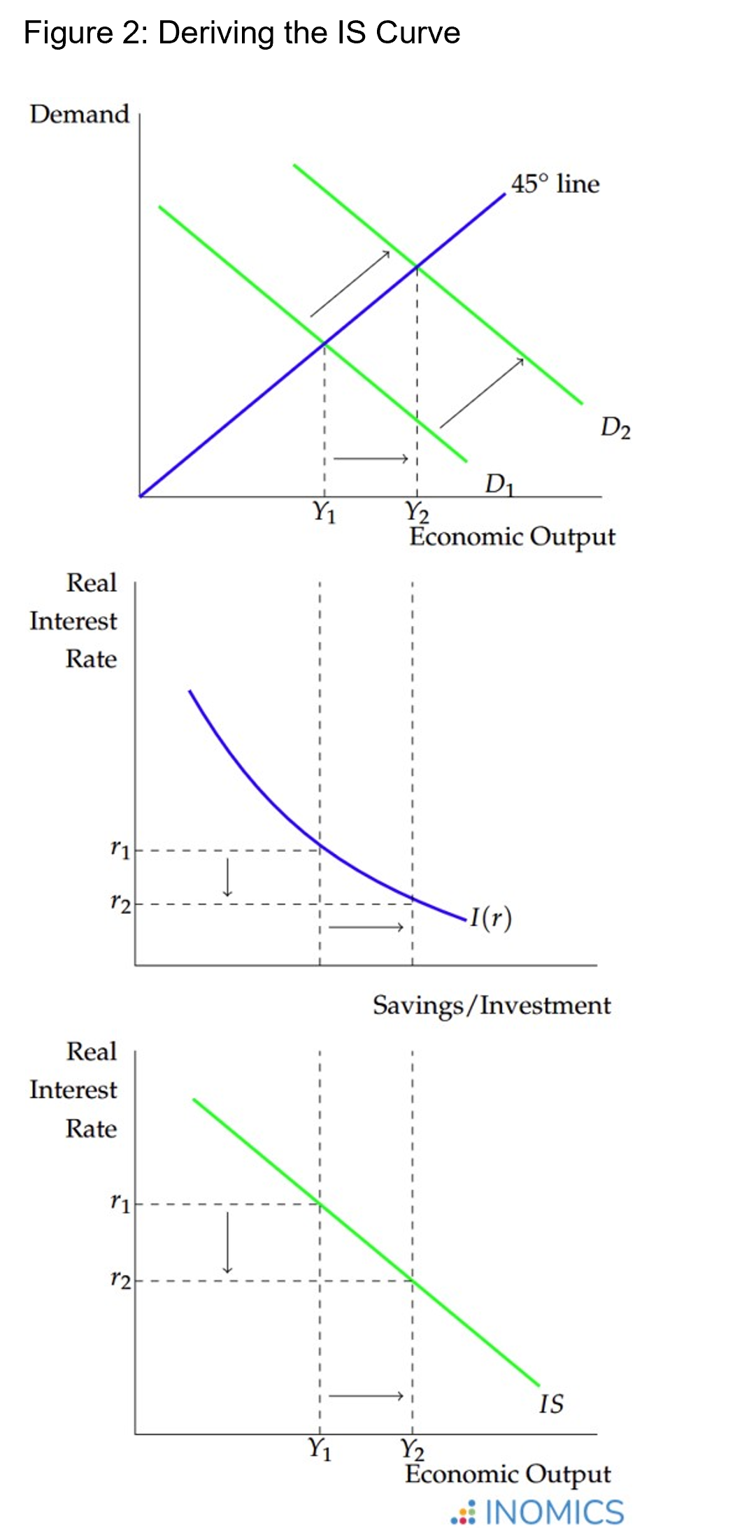
The top graph in Figure 2 depicts an economic expansion where an increase in demand led to higher economic output. Due to the higher output, the amount of savings (equivalently, investment) in the economy increases, represented by a movement along the I(r) curve in the middle graph. Because there is a higher demand for savings, the interest rate falls, since it represents the return on savings that banks pay out. These two realities – increased output and a decreased interest rate – are represented by a single movement along the IS curve in the bottom graph.

The IS curve is downward-sloping because as the interest rate falls, more investments are worth funding (remember that interest rates represent the cost of borrowing, too: in a falling interest-rate scenario, borrowing money is cheaper!). The increased amount of investments increases potential economic growth. Conversely, at a higher interest rate, fewer economic agents wish to borrow to fund productive projects; this decreases potential growth.

Taken from another perspective, the IS curve in economics also shows combinations of the real interest rate and output where the economy is in equilibrium, which in turn determines, or can be used to help anticipate, the level of aggregate demand.

The LM (Liquidity-Money) Curve

The LM curve shows where the money market is in equilibrium. At every point on the LM curve, liquidity preferences, income, and the real interest rate are such that the amount of money demanded is equal to the money supply.

Recall that the interest rate represents the return to savings, and therefore the “cost” of holding onto cash. As the interest rate increases, the demand for money decreases. Conversely, as income increases, money demand also increases.

To see why, suppose someone is holding $1000 in cash. This would feel like a lot of money for a college student with a limited income – but to a wealthy capitalist, $1000 is worth much less compared to the money they have available. It probably feels more like pocket change. Generally, when incomes (and by extension wealth) rise, money demand also rises.

The “liquidity preferences” part of the LM curve’s name reflects the amount of cash people are willing to hold in general, regardless of their income or interest rates. When people prefer to hold more cash, relatively speaking, the LM curve will be flatter (because it will take a larger increase in the interest rate to convince them to put their cash into savings), and vice versa.

Figure 3 shows the derivation of the LM curve from the money market equilibrium.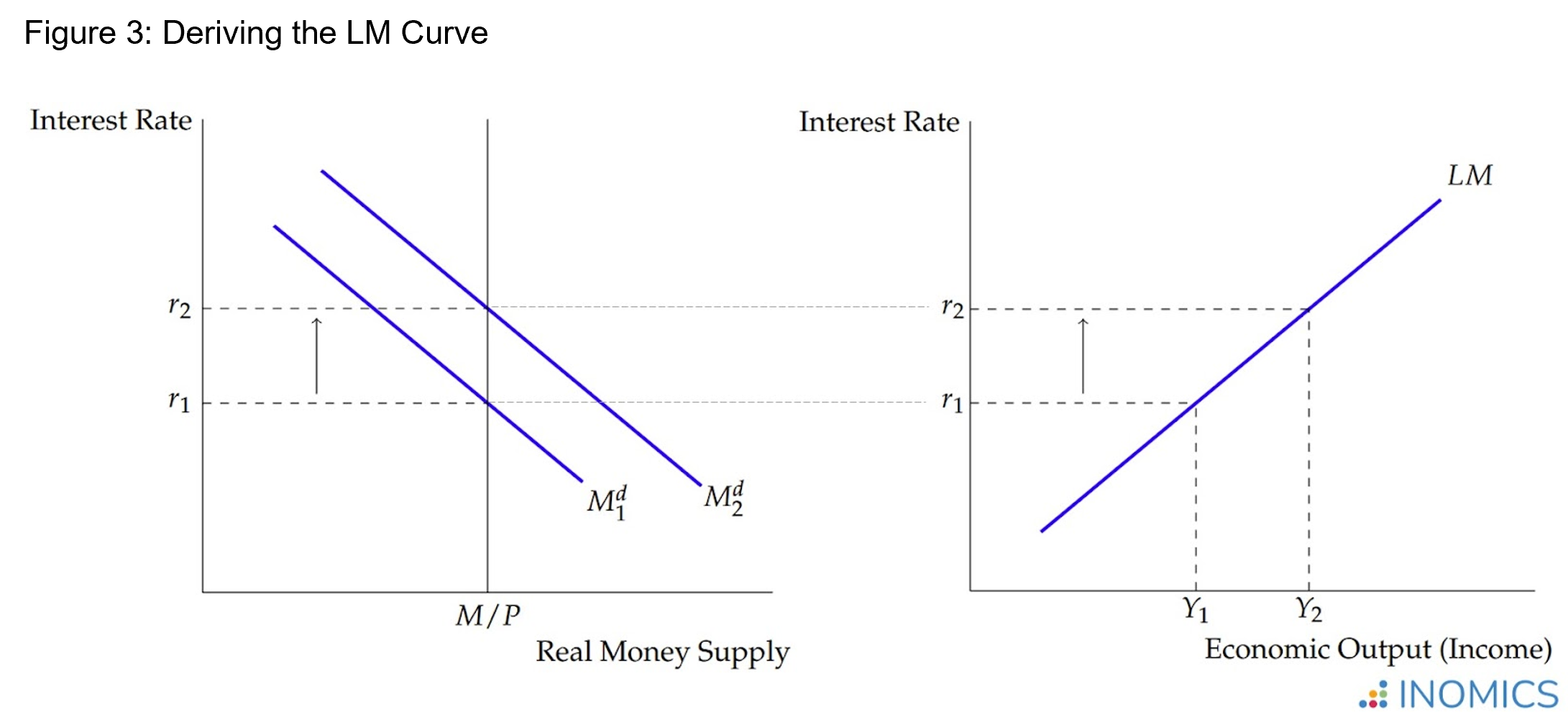

In Figure 3, the money demand curve slopes downward in the first graph because as the interest rate falls, there is less incentive to save money and less cost of holding cash. A shift in money demand (which can happen due to, for example, consumer preferences) shifts the interest rate in response.

Note that since the money supply is exogenously determined by the central bank (and commercial banks), Figure 3 determines the interest rate that will result from the central bank’s monetary policy and the amount of money demand. When the economy expands and GDP increases, money demand will shift upwards, increasing the interest rate at the fixed money supply. This is due to classic supply and demand dynamics; with a higher demand for money but the same supply, the “price” of holding money (the interest rate!) must increase.

The LM curve is upward-sloping in Figure 3, which is a facsimile of the curve in Figure 1. Note that on the left graph of Figure 3, the horizontal axis measures money demand/supply, but on the right side of Figure 3 (and in Figure 1) it measures income. Thus, the LM curve slopes upwards in Figure 1 because as income rises, money demand (and the interest rate) increases. This difference merely reflects a change in perspective, and should not be confused.

The IS-LM Equation

To consider the dynamics of the IS-LM model, it helps to look at the algebra behind both curves. The IS Curve is defined by the equation:

Y = C(Y – T(Y)) + I(r) + G + NX(Y)

where Y represents income (or output), C represents consumption, T shows taxes (as a function of income), I stands for investment, G is government spending, and NX is net exports. Students of macroeconomics will likely recognize this as very similar to the equations for aggregate demand and the expenditure approach of calculating GDP. But, there are a few key differences to discuss.

Often in mathematics, parentheses are used next to a variable to denote what factors determine the level of that variable. Here, then, the terms I(r) and NX(Y) show that here investment is a function of the real interest rate r, and net exports are a function of income Y. This makes sense; as income increases, people buy more goods, including goods from abroad (imports). And, clearly, the level of investment responds to changes in the real interest rate.

The C(Y – T(Y)) term shows that consumption in the IS curve is a function of both income and taxes (which itself is a function of income). This makes sense, too. The more income people have, the more they can spend and the more they’re taxed; and, taxes reduce discretionary income.

The equation for the LM Curve follows:

M / P = L(i,Y)

where M is the money supply, P is the price level (such that M / P shows the “real” money supply) and liquidity preferences L are a function of the nominal interest rate i and income Y. A specific functional form for the liquidity preferences equation isn’t given, but we know that it’s negatively related to the nominal interest rate and positively related to income (since people hold more cash as the interest rate declines and as income increases).

IS-LM Dynamics

Keeping these equations in mind shows clearly what economic phenomena will shift either the IS curve or the LM curve. Changes in one of the IS curve’s components – consumption, income, taxes, government spending, investment, or net exports – will cause a shift in the IS curve and therefore change the IS-LM equilibrium.

For example, consider a case where the government increases spending. While this must be funded by increases in taxes, which reduce consumption (in part due to crowding out), suppose that the multiplier effect is large and the increase in government spending ends up promoting growth. This increases income Y, and leads to an upward shift in the IS curve.

The increase in income is represented by the upward shift of the IS Curve, leading to a higher real interest rate at the new intersection with the LM Curve. The economy’s output grows as income rises, and the equilibrium interest rate is higher than before.

Suppose that, simultaneously, the central bank increases the money supply M such that M / P increases. This shifts the LM curve to the right, increasing output/income while reducing the interest rate.

Figure 4 shows a possible result of these changes.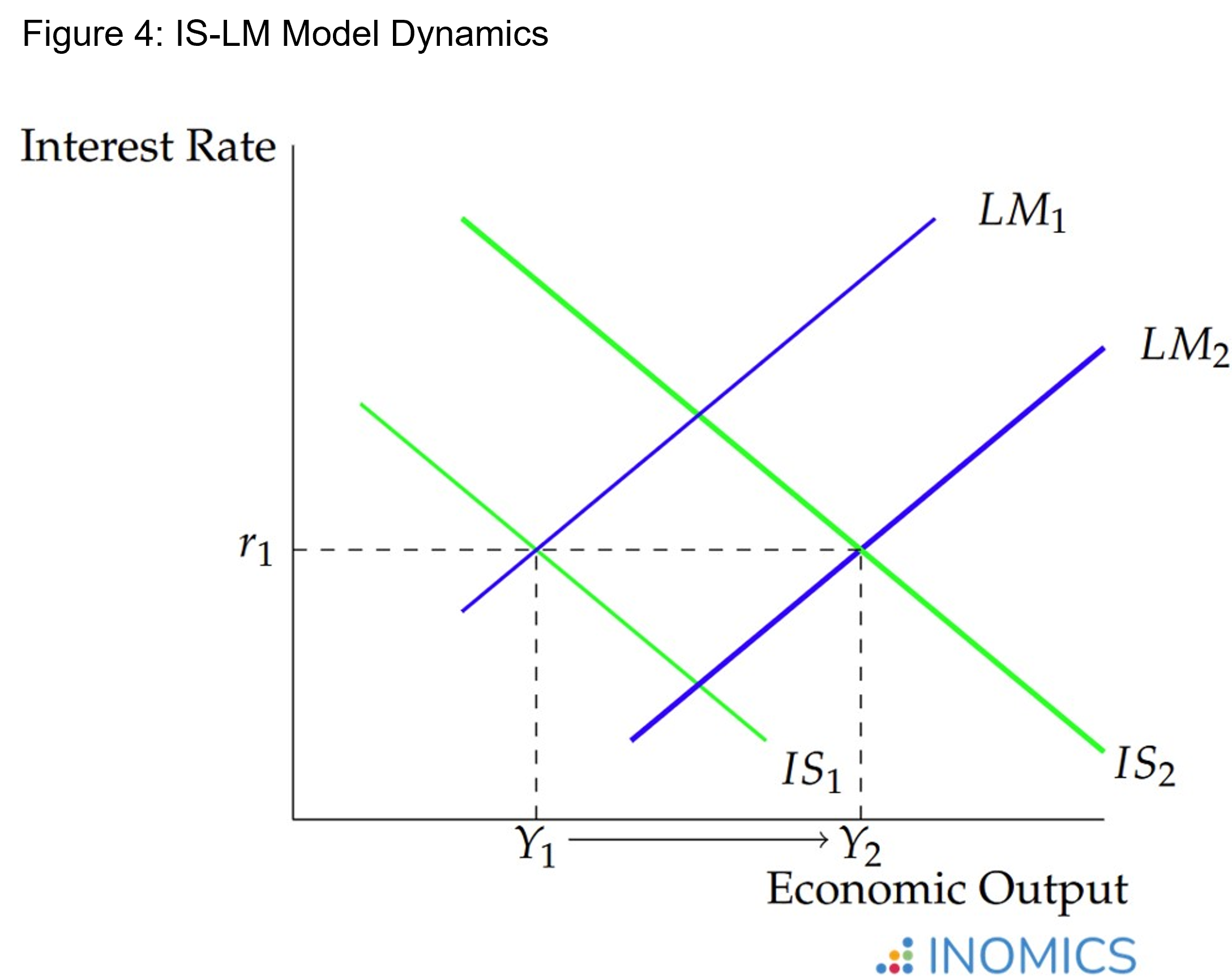

In Figure 4, after both curves shifted, the economy ended up with a higher level of output and an unchanged interest rate. Of course, it’s possible for the interest rate to be higher (if the IS curve shifts more than the LM curve) or lower (if the LM curve shifts more than the IS curve).

These simple examples represent two important levers for policymakers. The shift in the IS curve resulted from an act of fiscal policy, and the shift in the LM curve from an act of monetary policy. The usefulness of depicting these changes and predicting their outcomes led to the model’s former popularity.

Good to Know

However, the IS-LM model has fallen out of favor in recent years for several reasons. First, the model’s assumption that central banks focus on changing the money supply to affect the economy can be seen as outdated. Nowadays, central banks tend to focus on the interest rate itself (though there are notable exceptions to this, including “quantitative easing” policies in western economies prompted by the 2008 financial crisis) rather than the money supply, such that many economic models directly assume that the interest rate is set by the central bank.

Second, and very importantly, the IS-LM model assumes that the price level is constant. Notice how the price level P appears in the denominator of the LM curve equation, and is not considered a function of any particular variable (it is exogenous). Further, the real money supply is depicted as a vertical line in the money market.

It may seem strange now, since inflation is considered a critically important indicator of economic health, but until the 1970s (when stagflation reared its ugly head and stumped economists), it was much less of a concern for most policymakers. Obviously, this feature of the IS-LM model makes it unsuitable for studying inflation, and thus the model is unable to propose any policy solutions to combat inflation issues. This severely limits its usefulness, and macroeconomists have largely moved away from it.

Yet despite these fatal flaws, the IS-LM model is still widely taught in macroeconomics courses (though it tends to disappear in advanced macroeconomics). It’s a fundamental model that brings together many important concepts, and that undergraduates will certainly be tested on.