Economics Terms A-Z
Aggregate Demand
Read a summary or generate practice questions using the INOMICS AI tool
New students of economics quickly learn about supply and demand. These are foundational concepts in economics. Individuals prefer to buy goods at lower prices, and demand more of a good the cheaper it gets. Firms prefer to sell goods at higher prices, and supply more goods the higher the price for those goods.
This basic concept is applicable across all of economics, but is still mainly presented in a microeconomics sense. When deriving the demand curve in more advanced microeconomics courses, students will learn that the demand curve for an item (i.e., batteries) represents the summation of all individuals’ demand for that item in the economy.
In a similar vein, macroeconomics courses will eventually ask what happens if we sum all demand for all goods in the economy – by individuals, firms and the government? The resulting demand schedule (often represented by a curve) contains information about the general demand for all goods and services in the economy at various price levels, and is called aggregate demand.
Aggregate demand can be represented by a simple curve that looks just like an individual’s demand curve. Figure 1 shows an example. In the figure, AD and SRAS stand for “aggregate demand” and “short-run aggregate supply”, respectively. The short-run aggregate supply curve is the counterpart to aggregate demand, and is covered in its own article. Meanwhile, P represents the overall price level in the economy, and Y shows overall economic output.
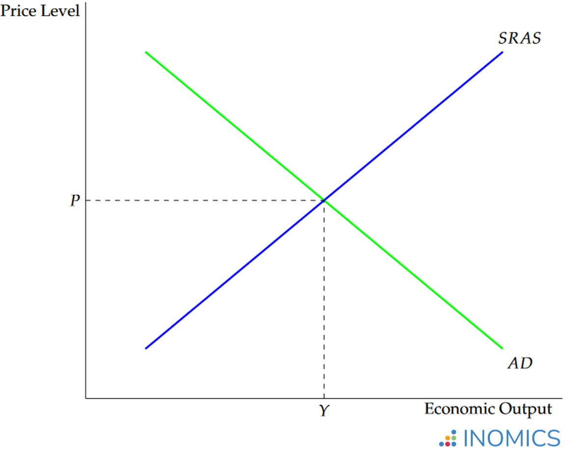
Figure 1: Example aggregate demand curve
Just as with the individual demand curve, the aggregate demand curve is downward-sloping. This is because economic agents (whether they are individuals, firms or the government) demand higher quantities of goods when those goods are cheaper.
The components of aggregate demand
Aggregate demand is defined mathematically as AD = C + I + G + NX. Here, C represents consumption spending by individuals and firms, I is investment spending, G shows government spending, and NX represents net exports. If any one of these components changes, ceteris paribus, the AD curve will shift.
C, consumption spending, may seem straightforward but is still worth examining. C includes all consumer spending in the domestic economy, as well as demand from firms for goods and services that do not constitute investment spending. When people buy household supplies, food, and movie tickets – or spend money on important services like healthcare and transportation – it’s counted towards C. When firms buy things like fuel, rented office space, or office supplies, it’s counted in C as well.
I stands for investment spending. Investment in this case refers to money used to purchase “capital goods”, which can include machinery, equipment, etc., forming one of the major factors of production. In other words, this is spending that will increase production, which increases Y – the economy’s potential output. Most of the time, this spending is conducted by firms that are seeking to expand operations. When an auto maker in Stuttgart, Germany decides to build a new factory, it’s counted in I, not C, in Germany’s aggregate demand. Other examples of I spending include land, machinery, infrastructure spending by the government, real estate purchases by rental companies, and more.
Another important component of I is research and development spending (R&D). This represents important research that can improve society, such as medical research, the development of advanced AI models, improved telecommunications technology, etc. R&D has more recently been recognized as part of I by many developed nations.
G shows spending by the government, which constitutes fiscal policy. This includes purchases such as infrastructure spending, hiring contractors for government jobs, education spending, etc.
Government spending may be controversial. Classical economists view government spending as most likely harmful since it will disrupt and distort markets through taxation, creating deadweight loss. Meanwhile, Keynesian economists believe that government spending can be key to bringing economies out of recession. This controversy is illustrated in more detail in the following section. Furthermore, government spending may cause crowding out; this is when government influence on the economy (whether via taxes or increasing demand) reduces private-sector investment spending.
The last term, NX, stands for net exports and may also be written as (X - M). In this case X represents exports and M represents imports (note that NX can be positive or negative depending on the trade balance). Notice what this implies about how aggregate demand accounts for foreign trade: AD includes foreign demand for domestic goods, but not domestic demand for foreign goods.
This makes sense. Consider Japan as the domestic country, which uses yen as its currency. When foreigners buy domestic goods from Japan, they spend money to acquire yen (probably in the foreign exchange market) and then buy Japanese goods. This increases demand for Japanese goods, boosts the Japanese economy, and strengthens Japan’s currency compared to others (increasing the exchange rate).
However, when residents of Japan buy foreign goods, they spend Japanese yen to acquire foreign currency and foreign goods. This weakens the yen compared to other currencies, and causes Japanese money to leave the country. Japan’s GDP would have been higher, ceteris paribus, had that money been spent in Japan and stayed within the country. If imports outweigh exports like this, NX will be negative in the equation above.
Shifts of the aggregate demand curve
The aggregate demand curve can shift, just like the demand curve can. The reasons why tend to be similar, but not exactly the same, because the aggregate demand curve measures demand in the entire economy. Demand shocks which affect one good may not affect the economy as a whole.
What does shift the AD curve, then? Changes in economic factors that affect one of the components of aggregate demand – C, I, G, or NX – will affect aggregate demand and shift the curve. Some common instigating factors include changes in wealth (for example, a fall in taxes increases wealth), the interest rate, and changes in business or economic expectations (also sometimes referred to as consumer confidence).
For example, if people become more pessimistic about the economy’s future – expecting a recession to hit – they will begin to prepare by saving more and spending less. This reduces C. Because C falls, the AD curve shifts inward and to the left in Figure 1. This lowers overall output Y, and can lead to deflation as the price level P falls. Ironically, people’s increasing pessimism becomes a self-fulfilling prophecy; aggregate demand continues to shift to the left as people cut back spending, which continually reduces output and thereby GDP, potentially leading to or worsening a recession.
Some economists (particularly the Keynesians) believe that an increase in G can help offset this negative feedback loop as it increases aggregate demand, potentially averting a recession by preventing AD from falling. Then, consumer expectations will reset, and the economy will remain at a healthy level of output. This scenario is one of the key arguments that economists may make in favor of an active fiscal policy.
However, astute readers may note that G must be funded by tax income. If consumers realize this, they may expect an increase in G to be accompanied by an increase in taxes, which may cause them to cut back spending even further. In fact, this is one argument often levied against employing an active fiscal policy. Macroeconomists, naturally, may debate whether a given fiscal policy is the right choice depending on the economic circumstances, political environment, sustainability concerns, or other factors.
Similarly to C, changes in I, G, or NX can shift the AD curve as well, and similarly may call for government intervention, a change in monetary policy, or nothing at all.
One thing that does not shift the AD curve, though, is a change in prices. Remember that both the demand curve and the aggregate demand show quantity demanded at any given price level; so, when the price level changes, one simply finds the corresponding quantity demanded on the original aggregate demand line.
Further Reading
Aggregate demand and aggregate supply form the basis of the AD-AS model in macroeconomics. This model marries together both concepts to describe a working model of the economy, and is used as an input to the more involved IS-LM model.
Good to Know
The price level, P, changes when the aggregate demand (or short-run aggregate supply) curve shifts. When there are positive shocks to aggregate demand, the curve shifts up and to the right, increasing Y. This is economic growth. However, there may be a catch.
When AD and Y increase, P increases as well! This causes inflation, and as we all know, too much inflation can be a bad thing for the economy. This is part of why economists may recommend increasing the interest rate to slow down the economy when there is an economic boom. It’s also a main reason why most economists consider pursuing expansionary monetary policy to be a mistake when the economy is doing well, as inflation will be pushed higher, which can be hard to bring down later without increasing the unemployment rate – even before accounting for the fact that policy often lags behind the true state of the economy, because it takes time to measure economic indicators and implement a policy.
-
- Assistant Professor / Lecturer Job
- Posted 1 week ago
Assistant (F/M) in the Research and Teaching Employment Group at Krakow University of Economics
At Krakow University of Economics in 3094802, Poland
-
- Assistant Professor / Lecturer Job
- Posted 1 week ago
Assistant Professor of Economics
At Marist University in Poughkeepsie, United States
-
- Postdoc Job
- Posted 2 weeks ago
Postdoctoral Research Fellow or Social Science Research Scholar at Stanford (USA) or Heidelberg University (Germany)
At Stanford University in Stanford, United States
Currently trending in United States

Related Items


Upcoming Deadlines
- Jul 29, 2026
- Jul 31, 2026
- Jul 31, 2026
- Aug 01, 2026
- Aug 01, 2026