The price elasticity of supply for an item A η_A measures how the quantity of the item supplied q_A changes in response to a change in the item’s price p_A

\begin{equation*}
\eta_A = \frac{\Delta\mathit{q}_{A}}{\Delta\mathit{p}_{A}} = \frac{\frac{d{q}_{A}}{\mathit{q}_{A}}}{\frac{d{p}_{A}}{p}}
    \end{equation*}

Price elasticity of supply is generally positive because firms are motivated to supply more (less) of an item as its price rises (falls). Precisely how sensitive supply is to changes in price depends on several factors. The most important is how long it takes sellers to adjust the amount of the item they can offer for sale. This is not just about the ability to ramp up production when more of the item is demanded. It is also about how feasible or costly it is for the seller to store items when demand falls.

The more complex the production process, the greater the dependence of sellers on other markets. Greater interdependence also increases the seller’s responsiveness to price changes. In markets for physical goods and the local provision of services, public infrastructure is also a significant factor in the price elasticity of supply.

The supply curves for five standard theoretical cases are shown in the graph below. In the first case, the supply curve S₁ starts at the origin (0,0), and is linear and upward-sloping. This implies that any change in price is met with a proportional change in quantity supplied. Therefore the price elasticity of supply is unitary η₁ = 1. If the item’s price increases by 10%, so too does its quantity supplied.

As with the price elasticity of demand there are two extreme cases for the price elasticity of supply: perfect elasticity and perfect inelasticity. The horizontal supply curve S₂ represents perfectly price-elastic supply: the elasticity tends towards (positive) infinity η₂ → ∞.

In theory, this means that if its price increases above p₂ then an infinite amount of the item will be supplied. But, if its price drops below p₂ then none will be supplied. Clearly, this is unlikely to happen in practice. However, in industries with flexible production and factor markets with spare capacity, the price elasticity of supply can be very high.

One example is the market for coffee-to-go. In this market, new entrants are very quick to take advantage of increased consumer willingness to pay, and leave the market quickly when conditions deteriorate.

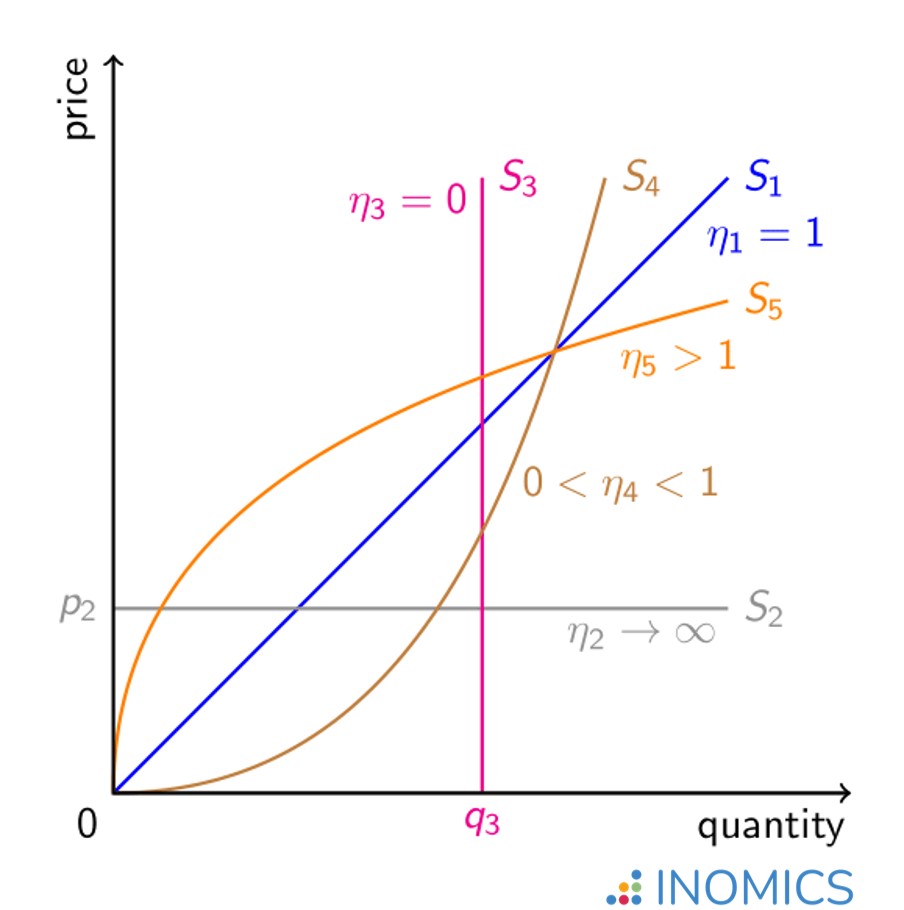
Figure 1: Various price elasticities of supply

At the other extreme, the vertical supply curve S₃ indicates that supply of the item is fixed at a quantity of q₃, whatever its price: supply is perfectly price-inelastic η₃ = 0. This is the case, at least in the short-term, for items with longer, less flexible production processes. Indeed, producers of such items are unable to react quickly to price changes.

The remaining two cases are the supply curves S₄ and S₅. The former represents relatively price-inelastic supply 0 < η₄ < 1. This can be seen by interpreting the graph: as the price increases, quantity increases only slightly. The latter shows a price elasticity of supply greater than unity η₅ > 1. In contrast to S₄, as the price increases, the quantity according to curve S5 increases by much more.

Economists distinguish between short-run and long-run supply curves due to the difference in their price elasticities. In the short run, supply is often assumed to be price-inelastic because the short run is defined by there being at least one fixed factor of production. In the long run, all inputs are variable and therefore supply tends to be more price-elastic, reflected in a flatter supply curve.

Further reading

The market for housing is a good example to gain an understanding of what can influence the price elasticity of supply. Using urban variation across the United States, Green, Malpezzi and Mayo uncover some key determinants of supply price elasticity in their article, “Metropolitan-specific estimates of the price elasticity of supply of housing, and their sources” (American Economic Review, 2005).

Good to know

The combination of price elasticity of demand and price elasticity of supply is what determines the respective sizes of consumer surplus and producer surplus in a market.

In general, the less price-elastic demand (supply) is, the greater the consumer (producer) surplus. This is particularly relevant information when it comes to market interventions  because it allows one to calculate which side of the market stands to gain most (or, more commonly, lose least) through a tax or other regulation on supply.