When the price ratio between items changes it can induce a change in consumption. There are two reasons for this. First, reducing the relative price of an item makes consumers more likely to purchase it when compared to other options (as long as they are normal goods or inferior goods, not Giffen goods or Veblen goods, which we assume in this article). Second, a consumer can now buy more of the item with the same amount of money. The first part, attributable to the change in the price ratio, is known as the substitution effect. The second part, the change in consumption that is brought about by the change in purchasing power, is known as the income effect.

Consider the graph below depicting two items, A and B, which are substitutes in consumption, i.e. an individual derives utility from both items and makes choices about how much to consume of each item depending on their relative prices. Initially, the consumer can afford up to Q_A of A or up to Q_B of B.

Depending on the individual’s preferences over items A and B, a series of indifference curves can be plotted. Along each indifference curve, the individual achieves the same degree of utility for the various combinations of items A and B. It is assumed that the individual seeks to maximize utility and that utility increases with consumption. Thus the individual will choose to consume the combination of items A and B at the point where the budget line Q_BQ_A is tangential to the indifference curve IC. Here, the individual initially chooses to consume q_A of A and q_B of B.

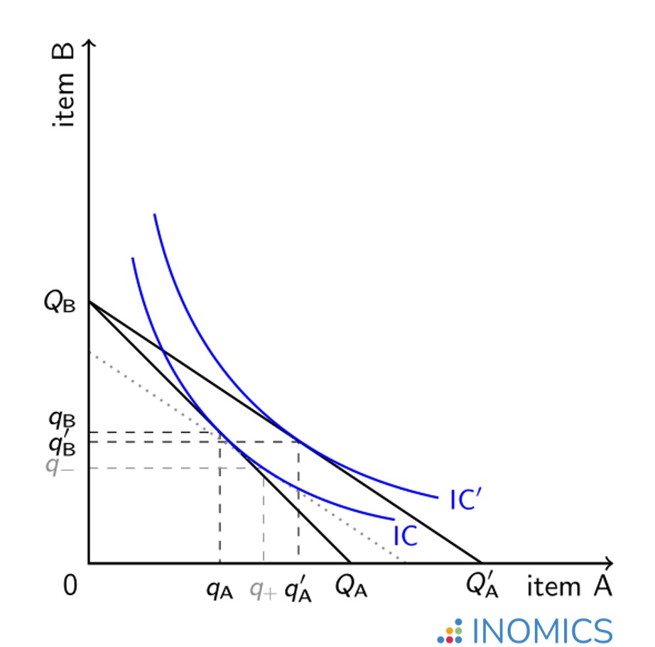
Figure 1: Illustrating the substitution and income effects from a change in budget

Now suppose that the price of item A falls such that if the individual were to devote all income to item A, Q_A’ of A would be consumed. The new budget line for the individual is Q_BQ_A’, a higher level of utility is attainable (indifference curve IC’) and the individual now chooses to consume q_A’ of A and q_B’ of B, which is the point where Q_BQ_A’ is tangential to IC’. Note how the individual’s consumption of item A has increased from q_A to q_A’, while consumption of item B has decreased from q_B to q_B’.

Because item A has become cheaper, the individual’s overall purchasing power has increased. Were the individual to continue to consume q_A of A and q_B of B in this new situation, they would have surplus income. Instead, in the grand quest to maximize utility, the individual moves from indifference curve IC to indifference curve IC’ for higher utility. The question remains, how much of the change in consumption from (q_A,q_B) to (q_A’,q_B’) is due to the change in the price ratio, and how much of it is due to the change in purchasing power?

Suggested Opportunities

• Master's Program
• (Online)
• Posted 3 days ago

Applied Economics (Banking and Financial Markets) online MSc

at University of Bath in Bath, United Kingdom

912996 90 University of Bath

• Master's Program
• Posted 1 week ago

Master in Economics - Barcelona

Starts 25 Sep at UB School of Economics, University of Barcelona in Barcelona, Spain

81660 81660 UB School of Economics, University of Barcelona

• Master's Program
• Posted 1 week ago

MSc Economics and Finance

Starts 2 Sep at University of Bath in Bath, United Kingdom

80 80 University of Bath

To answer this, consider how much of each item the individual would have consumed at the new price ratio but at the original level of utility (i.e. remaining on the original indifference curve IC). This can be worked out by drawing an imaginary budget line parallel to Q_BQ_A’ that is tangent to the original indifference curve IC. In the graph, this imaginary budget line is the gray, dotted line. We now see a greater decrease in the consumption of item B, from q_B to q–, and a lesser increase in the consumption of item A, from q_A to q+. This change in consumption from (q_A,q_B) to (q+,q–) is attributable purely to the change in the price ratio; it is the substitution effect (also known as the Hicksian substitution effect after the economist John Hicks).

Of course, the individual instead moves to the “better” indifference curve IC’ where (q_A’,q_B’) is consumed. A move from (q+,q–) to (q_A’,q_B’) is not due to a change in the price ratio. Rather, it is due to the change in the individual’s purchasing power brought about by one of the items becoming cheaper to consume. This is the income effect. Note how the income effect moves in the same direction as the substitution effect for the individual’s consumption of item A, while it does the opposite for the consumption of item B. The individual consumes more of item A both due to it replacing some consumption of item B and having greater purchasing power. However, the individual can also afford more of item B thanks to greater purchasing power, and thus the overall reduction in consumption of item B is dampened.

It is conceivable that the income effect dominates the substitution effect and vice versa for different types of items and different individual preferences and indifference curves. Indeed, the shape of the indifference curve is closely related to the cross (or cross-price) elasticity of demand, which describes whether and to what extent items are substitutes or complements in consumption.

Further reading

For an introductory analysis of substitution and income effects with intuitive explanations, see chapter 8 of Hal Varian’s textbook, “Intermediate Microeconomics: A Modern Approach”.

Good to know

Understanding substitution and income effects is also useful in the theory of production when the price ratio between inputs changes. Indeed, as technology progresses and machines become cheaper or more efficient in terms of their output, labor becomes a relatively expensive input. Firms may thus seek to replace workers with machines (substitution effect; see also the article on elasticity of substitution). However if the technology has improved then the firms should also be more profitable (income effect) and workers can lobby for the creation of better jobs or higher pay!