Economics Terms A-Z
Derivatives of Functions
Read a summary or generate practice questions using the INOMICS AI tool
Derivatives of functions are computed using differential calculus. A derivative in calculus is defined as “the rate of change of quantity y with respect to quantity x”. This sounds very similar to the definition for a slope, and in fact the derivative can be thought of as the slope of a curve. This article will discuss the usage of derivatives in economics, but will not explain how to calculate derivatives.
Derivatives are widely applied in economic modeling and theory, because they are an invaluable tool used to measure the effects and rates of change in economic variables and find the maximum and minimum values of functions.
Microeconomists and macroeconomists alike make frequent use of derivatives. The technique is key to solving constrained optimization problems, such as Lagrangian optimization, for the purposes of maximizing utility and profit. Many other decision problems can be represented mathematically and solved using first derivatives. Further, derivatives are often important for understanding why certain models of the economy differ or to examine their underlying assumptions.
Using derivatives in economics with a profit example
Consider the following production cost function for a good C(q) = k + aq2 where k is a fixed cost, q the number of units produced and a is a parameter representing variable costs. C(q) represents the total cost of production for q units of the good.
When making the decision about how much of the good to produce, a profit-maximizing firm will be interested in the cost of producing the last unit of the good (known as the marginal cost) and aim to set this equal to the extra revenue from selling that unit (marginal revenue). Suppose that (total) revenue from selling this good is simply the unit price p times the quantity sold R(q) = pq. Then profit (π) will be revenue minus cost π(q) = R(q) - C(q).
Maximum profit is found by taking the first derivative of the profit function and setting it equal to zero:
\[\begin{aligned} \frac{\partial\pi\left(q\right)}{\partial q}=\frac{\partial R\left(q\right)}{\partial q}-\frac{\partial C\left(q\right)}{\partial q}&=0\\ \Leftrightarrow\ \ \ \frac{\partial R\left(q\right)}{\partial q}&=\frac{\partial C\left(q\right)}{\partial q}\\ \Leftrightarrow\ \ \ p&=2aq\\ \Rightarrow\ \ \ q^{*}&=\frac{p}{2a}.\\\end{aligned}\]
Since the first derivative of the profit function is zero at this optimal point where p = 2aq, profits are neither growing nor falling. It can be verified that the point is a maximum (and not a minimum) by taking the second derivative of the profit function:
\[\begin{aligned} \frac{\partial^{2}\pi\left(q\right)}{\partial q^{2}}&=\frac{\partial^{2}\left(pq-\left(k+aq^{2}\right)\right)}{\partial q^{2}}\\ &=-2a,\end{aligned}\]
which is negative for positive a, i.e. the gradient (or slope of the tangent line) of the profit function is decreasing in q. In other words, as q grows, profits increase by a smaller amount, and beyond the optimal point q* profits begin to decrease as q increases further. So, profits are still growing at q < q* but falling for q > q* and therefore profits are at a maximum at q = q*.
This example is represented in the following graph where it is shown how profits (π) are maximized at point q = q* where the first derivative of the revenue function, which is marginal revenue, equals the first derivative of the cost function which is marginal cost (in other words, the point where MR = MC):
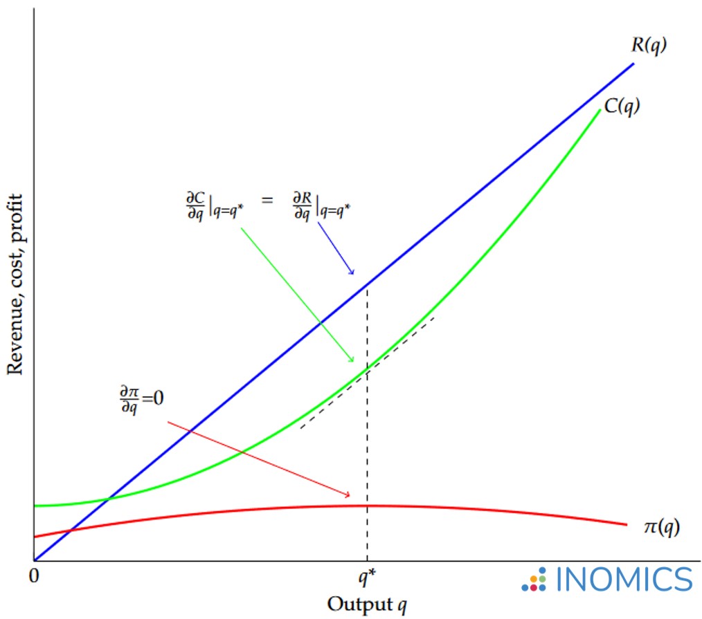
Figure 1: Graphical representation of profit maximization
In Figure 1, the red line shows the profit function. It is at its maximum at the point q*, which is also the point where the green cost function C(q)’s derivative (or slope of the tangent line) equals the slope of the blue revenue function R(q). Recall that this is the point where marginal cost equals marginal revenue.
Pointed out on the graph are the three relevant points on each function. Recall that profit is maximized at the point where the first derivative of the profit function equals zero. This is shown by the red arrow. This produces q* as the optimal quantity. It can be shown that the first derivatives of R(q) and C(q) are equal at this point by plugging q* into the provided functions and solving; these points are denoted by the blue and green arrows in the graph.
A note on total derivatives
The above example involves simple, direct, partial relationships between output quantity q and revenue/cost/profit. In most real-world situations, revenue and cost will also depend on other variables. For example, revenue is also affected by sales effort e and marketing expenditure m. Costs are additionally affected by the price of raw materials r and wages w. Insofar as these other variables interact with the production quantity, it may be necessary to calculate the total derivatives of the revenue and cost functions with respect to q in order to determine the optimal level of production,
\[\begin{aligned} \frac{dR\left(q,e\left(q\right),m\left(q\right)\right)}{dq}&=\frac{\partial R}{\partial q}+\frac{\partial R}{\partial e}\frac{de}{dq}+\frac{\partial R}{\partial m}\frac{dm}{dq};\\ \frac{dC\left(q,r\left(q\right),w\left(q\right)\right)}{dq}&=\frac{\partial C}{\partial q}+\frac{\partial C}{\partial r}\frac{dr}{dq}+\frac{\partial C}{\partial w}\frac{dw}{dq}.\end{aligned}\]
Calculating these total derivatives takes into account any indirect effects of changing the production quantity on revenue and cost that arise due to potential differences in sales effort, marketing expenditure, the price of raw materials and wages brought about by changing the production quantity.
Further reading
Hal Varian offers a simple introduction for economists on how to calculate derivatives of functions, both total and partial, in the mathematical appendix to his popular text book Intermediate Microeconomics: A Modern Approach (see sections A10 to A13 of the ninth edition).
Good to know
More often than not, when economists compute derivatives of functions they are performing ceteris-paribus analysis. Taking the partial derivative of a function y = f(x1) with respect to x1 is done to estimate the effect of x1 on y while assuming that all else remains equal.
This is why many economics courses only focus on the partial derivatives and assume that other influences on the revenue and cost functions remain constant. Therefore, total derivatives are seldom used in most economics courses. However, it’s still important to remember that basing economic reasoning on partial derivatives involves making the key assumption that other factors are held constant.
-
- PhD Candidate Job
- (Hybrid)
- Posted 4 days ago
Mehrere Doctoral Researcher (m/w/d) Für das Team "Forschung für die Finanzaufsicht"
At Deutsche Bundesbank in Frankfurt am Main, Germany
-
- Assistant Professor / Lecturer Job
- Posted 2 weeks ago
Assistant Professor - Economics
At Salisbury University in Salisbury, United States
-
- Event, Conference, PhD Candidate Job
- Posted 1 week ago
Tor Vergata Ph.D. Conference in Economics
At University of Rome Tor Vergata in Rome, Italy
Currently trending in United States


Related Items


Featured Announcements


Upcoming Deadlines
- Jul 26, 2026
- Jul 26, 2026
- Jul 29, 2026
- Jul 31, 2026
- Jul 31, 2026