AD-AS Model
Read a summary or generate practice questions using the INOMICS AI tool
There are a wide variety of macroeconomic models that aim to represent how economic activity works, and economics students will encounter many throughout the course of their studies. Arguably, the most common and important of these is the aggregate demand-aggregate supply model, or AD-AS model. Needless to say, you should be familiar with both aggregate supply and aggregate demand before continuing to read this article!
The AD-AS model uses the concepts of aggregate demand and supply to build a comprehensive model of the entire economy. While imperfect (like all models!), the AD-AS depiction is a great starting point when studying macroeconomic models; it can show the effects of just about any economic factor or shock on the economy. Importantly, the model also depicts inflation and output clearly, which in turn strongly hints at the level of unemployment, three important macroeconomic variables for any model to account for.
Full-employment output in the AD-AS model
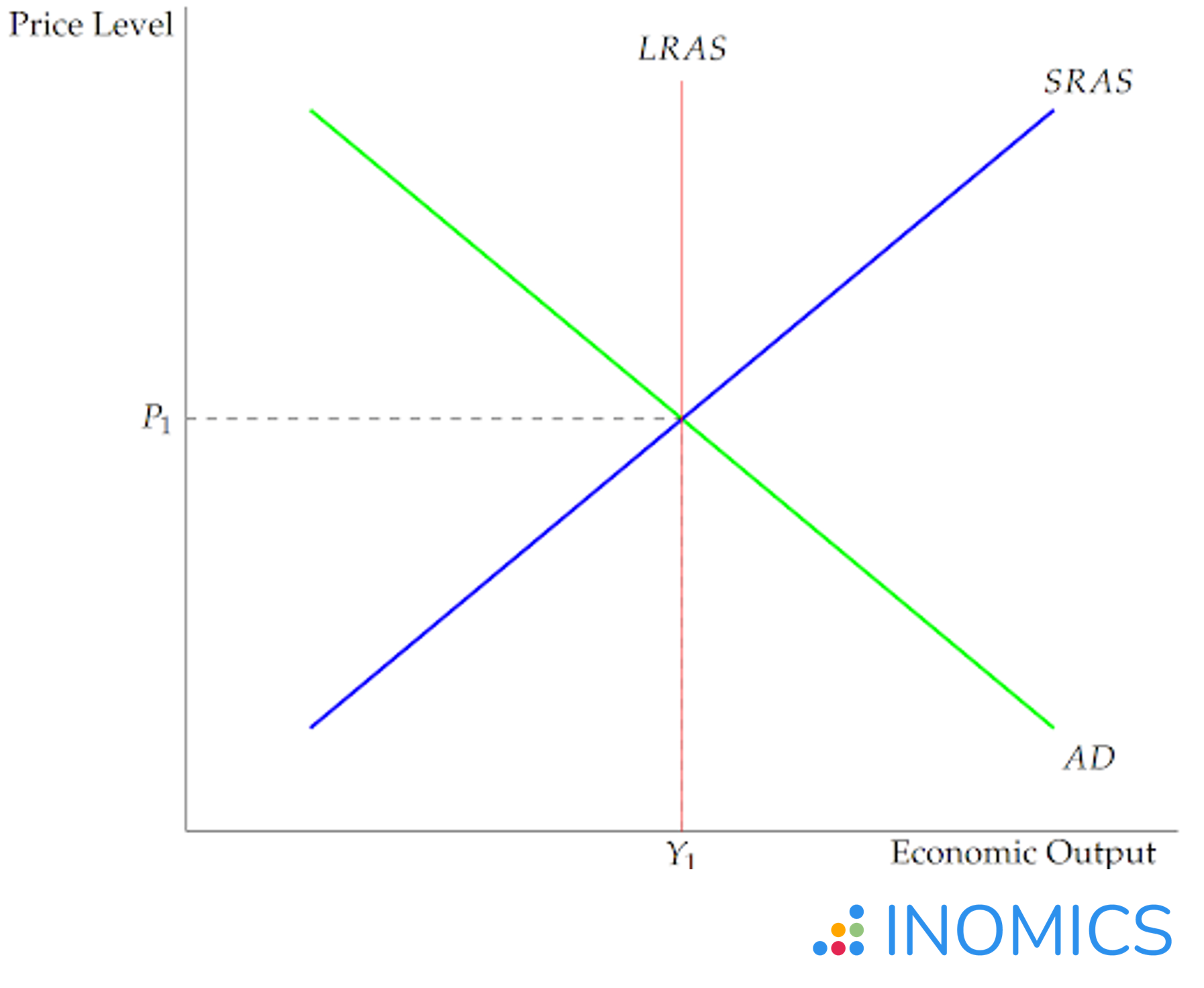
The basic form of the AD-AS model is shown in Figure 1. In this graph, equilibrium is at the point where the AD (aggregate demand) and SRAS (short run aggregate supply) curves intersect with both each other and the vertical LRAS (long run aggregate supply) line. This yields an equilibrium price level of P1 and output of Y1.

Figure 1: The AD-AS model in long-term equilibrium
When the economy is in this state, markets are in perfect harmony. We know this because when the three curves (AD, SRAS, and LRAS) intersect, the price level is steady, unemployment is as low as possible, and output (as measured by, say, GDP) is as high as is “safely” possible. At this three-way equilibrium, consumption and investment demands of consumers and businesses (AD) perfectly align with the production desires of suppliers (SRAS) at the current price level. In other words, the price level is steady because there is just enough supply to meet demand.
And, because the economy is efficiently using all of its resources (equilibrium is on the LRAS curve), we know that output is maximized. Because of this, we also know that workers are being utilized effectively and there is no unemployment (save for the unavoidable and healthy natural rate of unemployment). Thus, when short-term AD-AS equilibrium rests on the LRAS curve in the AD-AS model, the economy is in a state known as “full employment output”.
For deeper understanding, recall that the LRAS curve shows the maximum (healthy) potential output of the economy, and is unaffected by the price level. This is because the numeric price level doesn’t change how much real-world production factors – like raw materials, machines, and human intelligence – can actually produce. The LRAS curve, then, represents a Pareto-efficient usage of the economy’s resources.
In fact, the LRAS curve can also be thought of as a point on the economy’s Production Possibilities Frontier (PPF). When the economy is efficiently using all of its resources, it will reach a production mix on the edge of the PPF, and in the AD-AS model it will be at equilibrium on the LRAS curve.
Disequilibrium in the AD-AS model
This situation is all well and good, but the economy isn’t always in equilibrium! Let’s examine how the AD-AS model depicts disequilibrium.
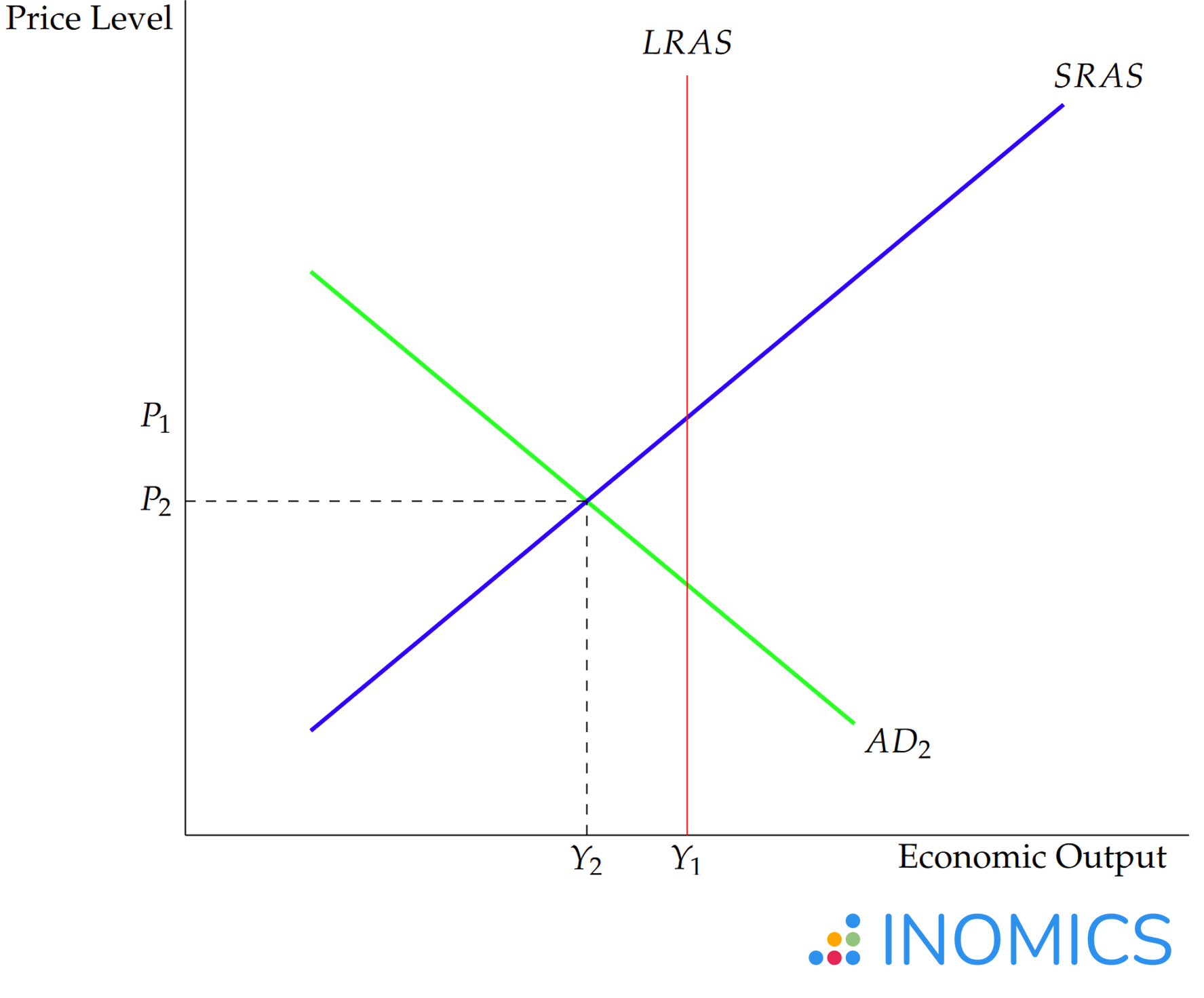
First, consider a situation where the short-run equilibrium – the intersection of AD and SRAS – lies to the left of the full employment level. What does this say about the economy?

Figure 2: The AD-AS model in recession
This shows that aggregate demand and short-run aggregate supply are in equilibrium, but they are not at the full-employment level of output depicted by LRAS. Since LRAS shows where equilibrium should be if the economy is utilizing its resources effectively, this economy isn’t producing output to its full potential – it’s producing at a point somewhere under the PPF curve.
It’s possible that the price level is too high, that there is too much unemployment, or that some negative shock occurred that made the economy less productive. In other words, Figure 2 is showing a recession!
In this specific case, notice how the AD curve has shifted to the left, and the new levels of prices and output are both less than in Figure 1.
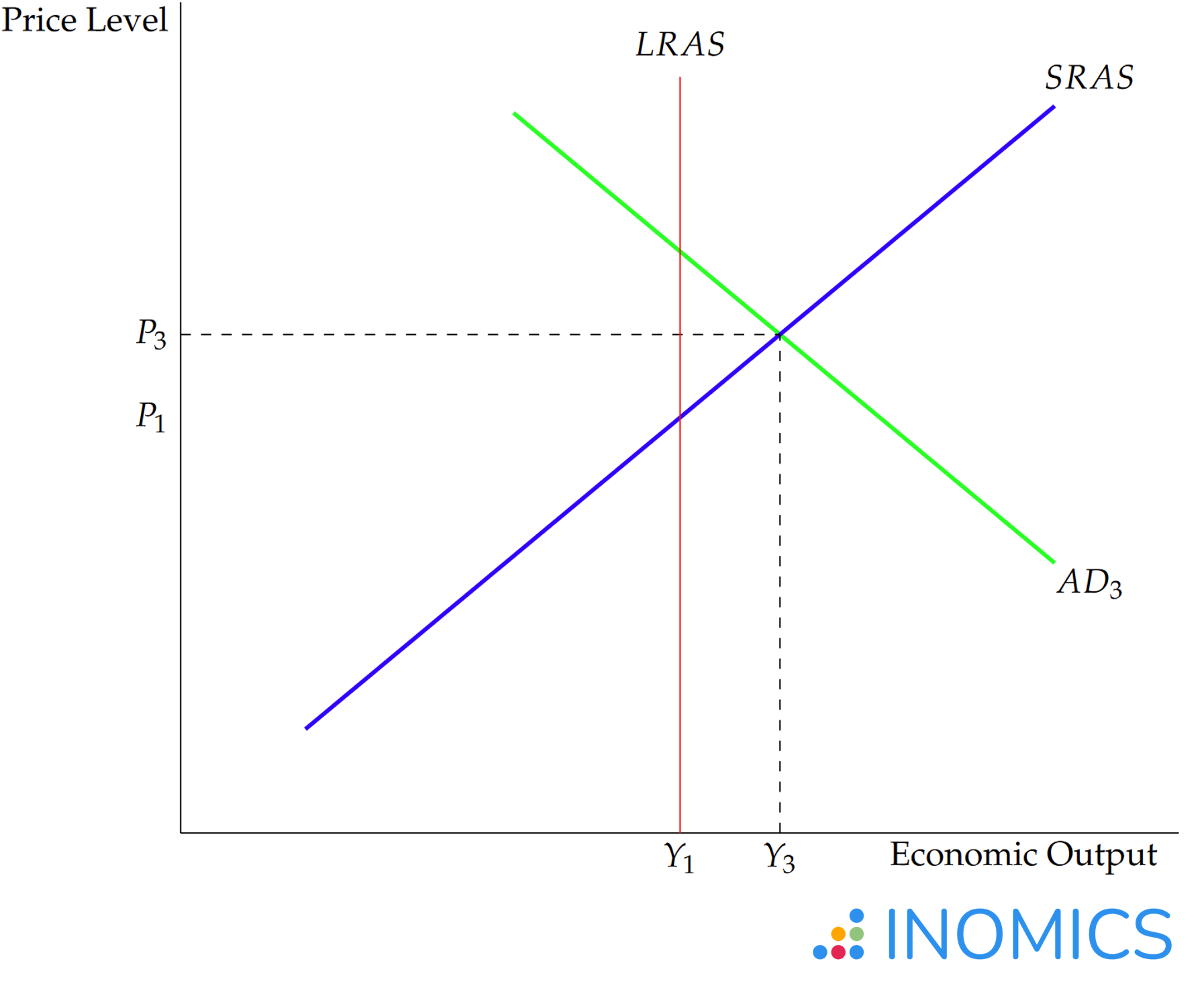
Figure 3 examines the opposite case – where the short-run equilibrium is to the right of LRAS.

Figure 3: The AD-AS model in an inflationary expansion
Now, AD and SRAS are at an equilibrium output greater than the full employment output. This is, in fact, possible. However, this isn’t some cheat code that heralds infinite economic growth; as with everything in economics and in life, there are no free lunches.
This inefficient overuse of resources comes with a serious cost: inflation! Notice how, compared to Figure 1, the AD curve has shifted to the right, leaving us with higher output and a higher price level.
The economy could be over-producing for several reasons, but in any case, free markets will eventually correct themselves. They will respond to the excess production by raising prices or reducing output, such that the new intersection of AD and SRAS returns to the LRAS curve.
One way this can come about is via an adjustment in the wage rate. Workers, noticing the increased productivity, will seek increased compensation. This upward pressure on the wage rate will eventually increase prices across the economy, as firms face higher labor costs, and by extension higher production costs. In this case SRAS shifts to the left, until it intersects AD at the point where both curves meet LRAS. The end result of the brief period of over-productivity, then, is the same long-run output as before, but at a higher price level.
This is just one way that inflation can occur as a result of Figure 3’s over-production. Regardless of the exact reasons, economists describe this state of the economy as an “inflationary expansion”.
That term – along with the terms “recession” and “full employment output” – define each basic state that the AD-AS model can be in, and tell us the position of the curves and likely state of the economy even without needing to see a graph.
Dynamics of the AD-AS model
Showing the state of the economy is helpful, but the true usefulness of the AD-AS model is that it can depict how the economy might shift into and out of equilibrium. In other words, it’s a tool that helps economists anticipate how real-world events will affect the economy, and why.
When examining the AD-AS model for these purposes, it’s important to remember the factors that can shift either the aggregate demand or aggregate supply curves. In Figures 1, 2 and 3, the AD curve shifted, but in the real world either AD, SRAS, LRAS, or even two or three of the curves can shift!
To recap, the equation for aggregate demand shows which factors can shift it:
AD = C + I + G + NX
(Where C represents consumption spending by individuals and firms, I is investment spending, G shows government spending, and NX represents net exports.)
If anything occurs that shifts one of its components, aggregate demand will shift. A full discussion can be found in the linked article.
Likewise, aggregate supply can shift too, and the linked article discusses how. The most common causes of a shift in aggregate supply include changes in the prices or availability of factor inputs, or changes in economic policy that make it easier (or harder) for firms to conduct business.
Long-run aggregate supply can also shift. When it does, it signifies a change in the economy’s total potential output. Innovation is a major factor that can shift LRAS to the right; destructive events like warfare or natural disasters can shift it to the left.
When any curve shifts, we can determine the likely effects on the economy using the graphs depicted in the last section.
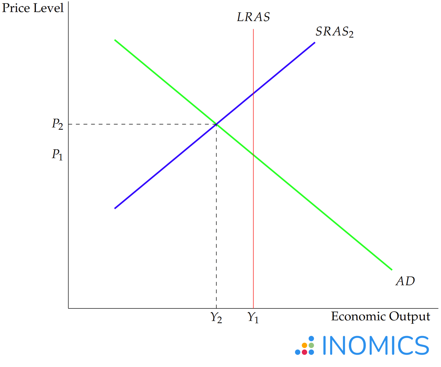
For example, suppose that a negative supply shock – such as an increase in the price of oil – hits the economy. This would cause SRAS to shift leftwards, as the cost of inputs is a major factor that can affect the supply of goods (LRAS does not shift in this case, since prices don’t affect long-run potential output). The leftward shift in SRAS corresponds to a movement left and up along the AD curve, bringing the economy to a new short-run equilibrium with lower output and higher prices – see Figure 4 below.

Figure 4: Recession caused by a negative shock to SRAS
But, in the long run, the economy will recover from the increased price of oil and return to its long-run efficient level of production. This can happen in many ways. In this example, it’s possible that the increased cost of oil incentivizes consumers and firms to find energy and input substitutes that don’t rely on oil. Suppose producers began to rely on solar power instead; eventually then, SRAS would return to the fully efficient level once firms had enough time to fully account for the increased cost of oil.
Multiple curves can shift at the same time, too. Consider a case where innovation in a domestic economy produces a major technological breakthrough – for example, suppose that one country alone invents desktop computers. This would improve economic productivity, shifting LRAS to the right; it would also (most likely) lead to a surge in foreign demand for domestically-produced computers, before other countries are able to begin producing their own supply. This increase in the NX term of aggregate demand shifts AD to the right as well. The final equilibrium is likely to be a scenario where the economy has both higher output and a higher price level, since LRAS and AD both shifted rightwards (representing a movement upward along the SRAS curve).
In these scenarios, the effect on the price level is clear. The likely effects on employment are easy to deduce from this model, too, although employment doesn’t appear explicitly on the graph. Consider the case just discussed, where LRAS and AD shifted rightwards. In response to the increased demand, firms would need to hire more workers and increase their capital stock, to increase production. Therefore, unemployment would most likely decrease.
AD-AS and the effects of policy
The articles on monetary and fiscal policy discuss the goals of the central bank and government when implementing policy. Generally, these institutions seek to boost the economy during times of recession, and slow the economy during times of (potentially inflationary) expansion.
It may seem odd at first to learn that these institutions might actually want to reduce or discourage economic activity. But, the AD-AS model immediately shows us when this can make sense. If the economy is in an inflationary expansion (like in Figure 3), it might be necessary to shift AD to the left so that the price level doesn’t increase too much. After all, runaway inflation can lead to difficult situations like stagflation or hyperinflation, especially if unforeseen events shift SRAS or LRAS to the left.
In order to affect the economy, the government can affect G (government spending) directly through fiscal policy. And, implementing laws and regulations can guide the economy in various ways, too. For example, if the economy is in a recession (like in Figure 2), cutting corporate taxes can shift SRAS to the right and encourage the economy to return to an equilibrium closer to the full-employment output level.
Monetary policy affects the AD-AS model too. To see how, first realize that the money supply can affect aggregate demand. If the central bank increases the supply of money, AD will shift rightwards (since consumers have more money to spend; or, alternatively, the velocity of circulation increases). This causes the short-run equilibrium to reach an increased level of output and prices (assuming that monetary neutrality does not hold). In times of recession, this is a policy lever that may seem quite appealing to bring short-run equilibrium back towards LRAS.
Depending on the country, the central bank also influences interest rates, which have important effects on the AD-AS model. Increasing interest rates encourages saving and discourages both consumption spending and (firms) borrowing to fund investment projects, which can shift AD leftward, and vice versa (nevertheless, the savings-investment identity continues to hold as the economy shifts).
Further Reading
The AD-AS model isn’t perfect, but it is a great starting point. Grasping this model will allow students to ace introductory macroeconomics courses, and build off of it to learn more complex models of the economy.
For an advanced discussion of the AD-AS model’s shortcomings, numerous papers are available. Consider, for example, David Colander’s The Stories We Tell: A Reconsideration of AS/AD Analysis. Yet, the model is still widely used in economics today because it is useful, relatively straightforward, and robust. See Amitava Krishna Dutt and Peter Skott’s Chapter 6 Keynesian Theory and the AD–AS Framework: A Reconsideration for an example of argumentation in favor of its continued use.
-
- Summer School
- Posted 2 weeks ago
CEMFI Summer School 2026
Starts 17 Aug at CEMFI in Madrid, Spanien
-
- Professional Training Course, Supplementary Course, Online Course
- (Online)
- Posted 4 days ago
Non-Linear Panel Data Models in Stata - Live Online Training Course
Starts 22 May at TStat Training
-
- Summer School
- Posted 2 weeks ago
Summer School - Seeing through the algorithms: a summer school on machine learning & AI for economists
Starts 6 Jul at UB School of Economics, University of Barcelona in Barcelona, Spanien


