Economics Terms A-Z
Aggregate Supply
Read a summary or generate practice questions using the INOMICS AI tool
New students of economics quickly learn about supply and demand. These are foundational concepts in economics. Individuals prefer to buy goods at lower prices, and demand more of a good the cheaper it gets. Firms prefer to sell goods at higher prices, and supply more goods the higher the price for those goods get.
This basic concept is applicable across all of economics, but is still mainly presented in a microeconomics sense. When studying the supply curve in microeconomics courses, students will learn that the supply curve for an item (i.e. batteries) shows how much of that item will be available for sale at any given price. At higher prices, more firms will seek to sell the item, and existing firms will seek to expand their production of the item.
In a similar vein, macroeconomics courses will eventually ask, what happens if we sum all supply for all goods in the economy? The resulting curve contains information about the general amount of all goods and services in the economy ready to be sold at various price levels, and is called aggregate supply.
Short-run vs. long-run aggregate supply
Unlike with its counterpart aggregate demand, aggregate supply can’t easily be represented by a single curve. To analyze aggregate supply, it’s important to distinguish the time period considered. This leads us to have two main aggregate supply curves: “short-run aggregate supply”, or SRAS, and “Long-run aggregate supply” or LRAS.
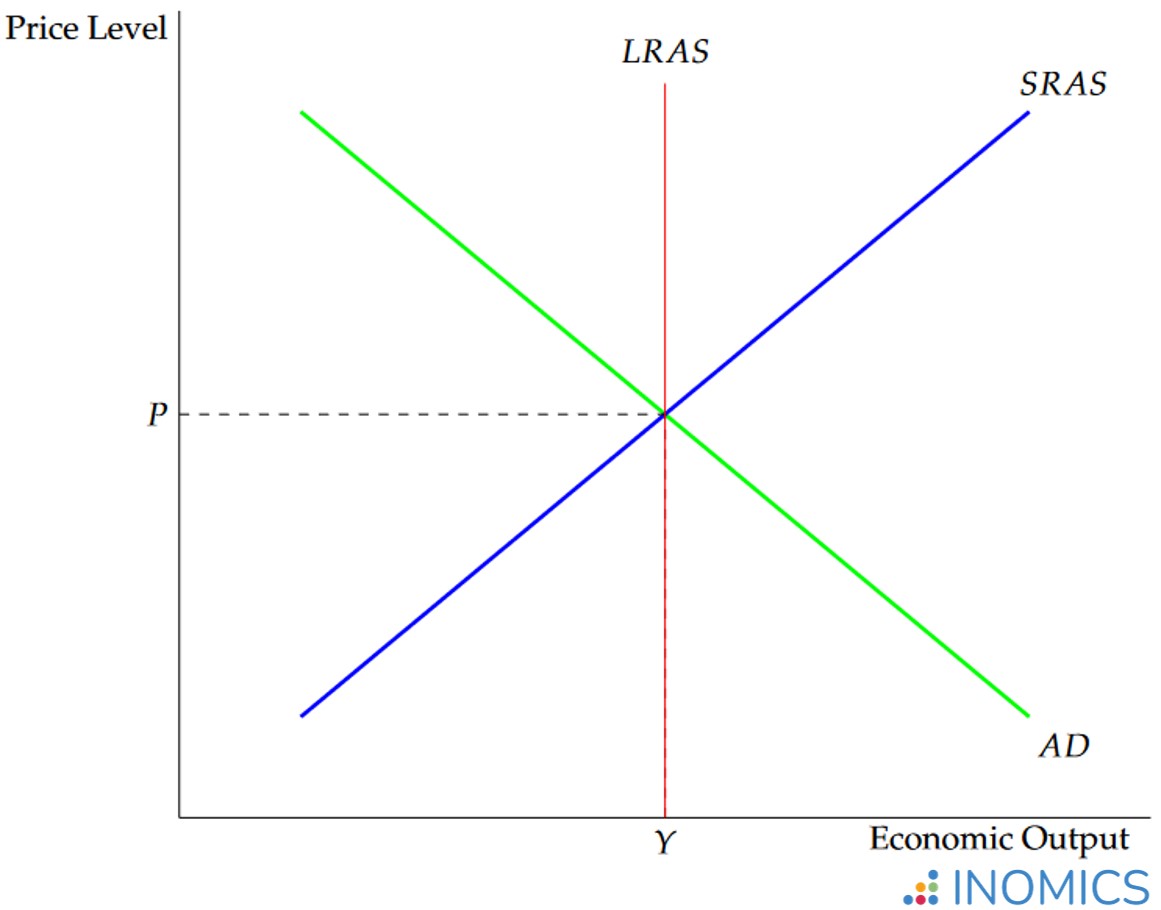 Figure 1: example aggregate supply curves
Figure 1 shows an example. In the figure, P represents the overall price level in the economy, and Y shows total output (often measured by GDP). Meanwhile, AD and SRAS stand for “aggregate demand” and “short-run aggregate supply”, respectively.
SRAS is upward-sloping and can be thought of similarly to a traditional supply curve considered from a microeconomics sense, though there are important differences. It is upward-sloping because firms are willing to sell higher quantities of goods when those goods can be sold at a higher price. Meanwhile, AD is downward-sloping like an individual’s demand curve, though it is distinct. See the aggregate demand article for more detail.
Finally, LRAS in Figure 1 stands for “long-run aggregate supply”. Unlike supply curves students first encounter, this one is vertical. In other words, for all values of the price level P, the output Y is not changed.
In the short run, prices matter
SRAS may be easier to understand at first than LRAS, for the simple reason that it behaves much like a typical individual’s supply curve that students usually already know. When prices in the economy rise, producers believe that they can make more profit if they increase production, so they do. When prices fall, producers can’t sell as many units profitably. Consider that producers sell units up to the point where marginal cost equals marginal benefit. When price falls, it lowers marginal benefit (in this case marginal revenue), so producers must sell fewer units or make losses.
At this point, classical economists would argue that changing prices do not affect firm decisions, or any real variables such as the profit-maximizing unit. In the classical view of the economy, price changes are instantly spread throughout the economy and accounted for by everyone, and so do not affect these decisions. So, in a classical model, the SRAS curve would not be upward-sloping (in fact, it would be vertical just as the LRAS curve is).
One argument levied against this classical view is that real-world experience shows that some prices and costs, especially wages, are often sticky. That is, firms don’t – and often legally can’t – change wages at a whim. These “sticky wages” support the idea that in the short term, price changes do have an effect on firm decisions.
Remember that wages are paid to labor, which is an important factor of production, and represents a large proportion of most production costs. Consider a fall in prices. This reduces the profit, ceteris paribus, of the firm (in a perfectly competitive market, the fall in prices means the firm must produce fewer units or lose money, for the reasons discussed above). It would be optimal for the firm to reduce some of its production costs if it can, to offset the lower sales price and regain some of that lost profitability.
However, wages are often set by contracts and cannot be easily reduced – not to mention that trying to reduce wages is a great way to dismay valuable employees and ruin morale. Therefore, firms cannot reduce their costs enough to make up for the reduced price of their goods. Thus, they end up cutting some production to prevent losses. Conversely, because wages are hard to lower and firms don’t want to unnecessarily raise their costs, firms may hold off on increasing wages when prices rise.
Menu costs are another reason that price changes may not adjust immediately, and therefore can cause short-term fluctuations in economic activity. Consider a traditional sit-down restaurant that wishes to change prices. In order to change prices, the restaurant will have to re-print the paper or plastic menus that it hands to its customers. This costs money, so it’s only worth doing once the benefits from updating the menu prices outweigh the costs of printing new menus – meaning prices may take some time to adjust. Menu costs can apply to other things as well – such as updating software to include new prices, or conducting market research to find the best new prices before changing them.
Menu costs and sticky wages are easily observable in most economies today. But this does not disprove classical economic theory. Neoclassical economists have updated classical economic models to account for modern concepts like sticky wages and menu costs – economists are always learning!
Regardless, in the long term prices are considered fully flexible no matter which school of thought an economist might subscribe to. Wages will be renegotiated, menus will have been updated, and economic agents will adjust to the new prices. Therefore, as the classical economists posit, economists tend to agree that eventually the price change no longer affects economic output or profitability.
Shifts in short-run aggregate supply
As usual, changes in the price level do not move the SRAS curve; they represent movements along the curve, not of it. The factors that shift SRAS are economic events that change the firm’s production decisions for any price level. In other words, SRAS shifts when a new economic situation changes the optimal production level regardless of the price level. This can be the case when the economy becomes more or less productive, when the prices of factor inputs change, and other events that change the profit per unit for producers.
Consider advancing technology, usually represented by A in the classic Cobb-Douglas production function. As technological progress continues, eventually there is an invention or an improvement that increases productivity. For example, the invention of the printing press greatly increased the economy’s ability to produce books. This invention led to a decrease in the overall cost of producing a book and increased literacy as reading became more important. These factors in turn increased productivity even more.
Incidentally, the printing press also led to the obsolescence of scribe work. Becoming a professional scribe is no longer a valid career option for the majority of people, since we can easily create and print written works without the need for handwriting or physical labor. This process of technology and productivity growth eliminating some jobs (while creating others) is known as creative destruction in economics. While some jobs are lost due to creative destruction, overall this phenomenon leads to a more productive economy and an overall better standard of living for everyone.
Such an increase in productivity – even if it results in the loss of some jobs or even entire industries – causes the SRAS curve to shift to the right. Likewise, a reduction in productivity will cause SRAS to shift to the left. Because the economy has become more productive, firms are generally able to produce “more with less”. Profit per unit increases, causing firms to want to produce more at any price level.
One important point to note before moving on is that changes in the prices of intermediate goods are not considered to be changes in the overall price level. The reason for this is similar to the reason economists don’t include intermediate goods in the calculation of GDP; the prices of intermediate goods are factored into the final output that firms produce. So, to avoid double-counting them, the overall price level represents only the prices of final goods (just as GDP calculations only consider the value of final goods).
Therefore, changes in the prices of factor inputs – such as wages, or factor input commodities like oil – will cause changes in the profit per unit calculation that employers make, but won’t change P. This changes the profitability per unit and shifts firms’ preferred production at any given price level. Finally, this results in a shift of the SRAS curve.
Conversely, a change in the sales price of the firm’s output will cause a change in P. This then requires the firm to find the newly optimal production mix at the intersection of SRAS and AD.
Shifts in long-run aggregate supply
The LRAS curve can shift, too. Recall that LRAS is the long-run output of the economy and is not affected by the price level. How, then, does it shift?
Anything that affects the economy’s total potential output Y will shift the LRAS curve, since LRAS = Y for any P. One common reason for this is a change in the business cycle – “booms” shift the LRAS curve to the right, increasing potential output Y. Meanwhile, “busts” or recessions shift the LRAS curve to the left, decreasing potential output.
Because LRAS = Y for any P, changes in the price level do not have an effect on potential output. This makes sense, as the prices of items in the economy are essentially arbitrary numbers. Prices have meaning only in the context of other prices. Therefore, tripling all prices in the economy, while at the same time tripling the amount of money everyone has, will (theoretically) have zero effect on economic activity.
One way to think about this: people ultimately exchange real economic value (the product of their labor, paid in wages) for real economic goods. Money is simply acting as a medium of exchange during that process, and so the money supply does not itself affect real economic variables. The theory of monetary neutrality explores this idea in greater detail.
It’s possible for both SRAS and LRAS to shift from the same economic shock. An improvement in technology that increases economic efficiency has the potential to increase both curves. Firms can be positively impacted by this technological change in the short run, increasing output to take advantage of the increased productivity (shifting SRAS to the right). Meanwhile, the increased efficiency the technology introduces permanently increases the potential output of the economy, shifting LRAS to the right.
SRAS and LRAS lead the economy to a stable equilibrium over time
It’s possible for the economy to be at an equilibrium where AD and SRAS intersect, but not LRAS. If this equilibrium output is below LRAS, this situation is a recession. If it’s above LRAS, it’s a potentially inflationary expansion.
This process is described by the AD-AS model in macroeconomics.
Further Reading
The aggregate demand curve and aggregate supply curves form the basis of the AD-AS model in macroeconomics. The model marries together both concepts to describe a working model of the economy.
Many of these concepts also appear in the IS-LM model, another major model that students of macroeconomics will need to learn. Both AD-AS and IS-LM describe how the economy reaches macroeconomic equilibrium.
Good to Know
The LRAS line also represents the economy’s potential output, often denoted YP. This is the potential output of the economy under a scenario of “full employment”, where all resources (including labor) are being used in an economically efficient manner.
This means that the LRAS curve also represents a point that lies on the economy’s production possibilities frontier. Recall that in the PPF, each point on the curve represents a point where the economy is functioning in a Pareto efficient manner, where all resources are being utilized productively to their fullest potential.
-
- Researcher / Analyst Job
- (Hybrid)
- Posted 1 week ago
Wissenschaftliche:r Mitarbeiter:in Metascience in Economics
At ZBW Leibniz Information Centre for Economics in 2911298, Germany and Kiel, Germany
-
- Assistant Professor / Lecturer Job
- Posted 2 weeks ago
Assistant Professor - Economics
At Salisbury University in Salisbury, United States
-
- Postdoc Job
- Posted 1 week ago
Postdoctoral Research Fellow or Social Science Research Scholar at Stanford (USA) or Heidelberg University (Germany)
At Stanford University in Stanford, United States
Currently trending in United States

Related Items


Featured Announcements


Upcoming Deadlines
- Jul 26, 2026
- Jul 26, 2026
- Jul 29, 2026
- Jul 31, 2026
- Jul 31, 2026