Economics Terms A-Z
Cournot Competition
Read a summary or generate practice questions using the INOMICS AI tool
Cournot competition describes an oligopoly market model in which two or more firms produce the same good and compete for market share. The competing firms decide simultaneously and independently of each other on the amount of output they will produce. The total quantity supplied by all firms then determines the market price. This is distinct from Bertrand competition, where firms compete in prices, or Stackelberg competition, where firms sequentially choose their production quantities.
The French polymath Antoine Augustin Cournot (1801–1877), after whom this economic model is named, illustrated this market situation using the example of two firms exploiting mineral water springs, each able to produce unlimited quantities at zero cost.
According to the law of demand, there is an inverse relationship, or negative correlation, between quantity and price. That is, higher levels of production result in relatively lower prices, and vice versa. To maximize profits, each firm has to consider this trade-off between quantity and price, taking the expected market supply by its competitors into consideration.
This constitutes a game strategic situation (see also game theory). In the Cournot-Nash equilibrium, each firm chooses the quantity that presents the ‘best response’ to the competitor's production quantity.
Below we derive the Cournot equilibrium quantities and calculate the market price. We will see that Cournot competition leads to a more efficient market outcome than if there was only one firm in the market (monopoly). But, there is still an efficiency loss compared to the equilibrium under perfect competition.
Model Assumptions
Let's have a quick look at the main assumptions of the Cournot model:
- There is a fixed number of firms in the market and firms have market power. This means that each firm's production decision affects the market price.
- All firms produce a homogenous good. In other words, there is no product differentiation. This means that the goods produced by any firm are completely identical in the eyes of the consumers (they are perfect substitutes).
- Firms compete in terms of the quantities that they produce. That is, they compete for market share. This is the key difference to Bertrand competition, in which firms compete in prices.
- Each firm acts strategically on the assumption that its competitor(s) will choose the equilibrium quantity, and decides its own production quantity so as to maximize its profit.
- The production decisions by all firms are made simultaneously. This is the key difference to Stackelberg competition, in which the leader firm moves first and then the follower firms move sequentially.
- Firms do not cooperate.
The Cournot-Nash equilibrium
To derive the Cournot-Nash equilibrium, we will focus on the example of a duopoly. That is, there are only two firms in the market. We will assume that firms 1 and 2 both produce the same good at the same production cost c1 = c2 = c.
We assume demand is a linear function given by p(Q) = a - bQ where a > 0 and b > 0. If one firm produces q1 and the other produces q2, then the total market quantity is Q = q1 + q2. So, we can substitute this expression for Q in the following equations. Firm 1's total revenue is then given by the market price times the quantity produced:
\begin{equation*}
r_1=pq_1=(a-b(q_1+q_2))q_1 \quad \text{(analogous for firm 2)},
\end{equation*}
and firms 1's total profits are calculated as the difference between revenue and production costs:
\begin{equation*}
\pi_1= pq_1-cq_1=(a-c-b(q_1+q_2))q_1 \quad \text{(analogous for firm 2)}.
\end{equation*}
From here we will assume a > c, which is a necessary condition such that positive profits can be realized.
Each firm then chooses the production quantity that maximizes its profits, taking the quantity produced by its competitor into consideration. So, to derive the optimal output, we need to find the quantity q1 that maximizes the profit function for firm 1, taking q2 as given. Analogously, we will do the same for firm 2. To find the optimum, we take the partial derivative of the profit function and set that equation equal to 0:
\begin{align*}
\max_{q_1} \{\pi(q_1) &=(a-c-b(q_1+q_2))q_1\} \\
\frac{\partial \pi(q_1)}{\partial q_1} &= a-c-2bq_1-bq_2 = 0 \quad | \quad \text{solve for q1} \\
q_1^* &= \frac{a-c-bq_2}{2b} \\ \text{and analogously} \quad q_2^* &= \frac{a-c-bq_1}{2b}.
\end{align*}
The equations q1*(q2) and q2*(q1) are called the best response functions. They tell us firm 1's optimal output for any quantity produced by firm 2, and firm 2's optimal output for any quantity produced by firm 1.
In the Cournot-Nash equilibrium, both firms will give their best response to each other's actions. To derive the equilibrium, we thus insert the optimal response of firm 2 into firm 1’s equation to calculate its optimal quantity, and vice versa:
\begin{align*}
q_1 &= \frac{a-c-b\frac{a-c-bq_1}{2b}}{2b} \quad | \quad \text{solve for q1} \\
q_1^* &= \frac{a-c}{3b} \\
\text{and analogously} \quad q_2^* &= \frac{a-c}{3b} = q_1^*.
\end{align*}
This is the unique Nash equilibrium for the Cournot duopoly. Entering the optimal quantities into the demand function gives us the total quantity and the market price in the equilibrium:
\begin{align*}
Q^* &= q_1^* + q_2^* = \frac{2}{3} \left[\frac{a-c}{b}\right] \\
p^* &= a - bQ^*= a - \frac{2}{3}(a-c) = \frac{a+2c}{3}.
\end{align*}
Graphically, the equilibrium point E is where the best response curves q1*(q2) and q2*(q1) intersect. The figure also illustrates the quantities q1M and q2M that would have been produced if either firm 1 or firm 2 was the only one operating in the market; that is, if either firm had full monopoly power.
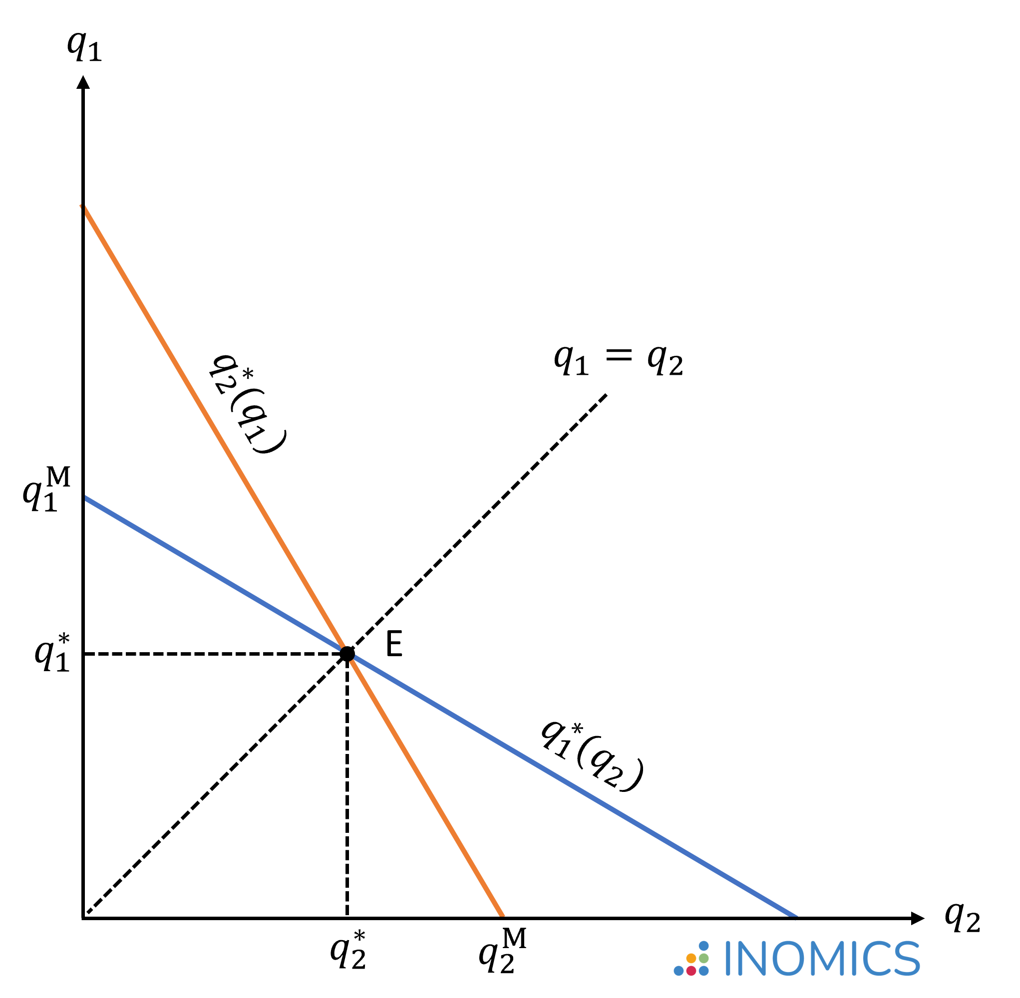
Figure 1: Cournot-Nash Equilibrium
We can also use the model solution derived above to compare the monopoly and Cournot duopoly situations. If we assume that firm 1 is the only producer, this implies q2 = 0 and thus:
\begin{align*}
q_1 &= \frac{a-c-bq_2}{2b} \quad | \quad q_2=0 \\
\Longrightarrow q_1^M &= \frac{a-c}{2b}=Q^M \\
\text{and} \quad p^M &= a - bQ^M= a - \frac{1}{2}(a-c) = \frac{a+c}{2}.
\end{align*}
From this we can conclude that in the duopolistic Cournot-Nash equilibrium, the total quantity of output produced is larger and the price is smaller than in the monopolistic market equilibrium:
\begin{align*}
Q^* &= \frac{2}{3} \left[\frac{a-c}{b}\right] > \frac{1}{2} \left[\frac{a-c}{b}\right]=Q^M \\
\text{and} \quad p^* &= \frac{a+2c}{3} < \frac{a+c}{2} = p^M \quad \text{if} \quad a>c.
\end{align*}
However, there is still a welfare loss compared to the market equilibrium under perfect competition. In a perfectly competitive market, price equals marginal cost and firms earn zero profits, thus pC = a - bQC = c. From this we can conclude that in the duopolistic Cournot-Nash equilibrium, the total quantity of output produced is lower and the price is higher than in the competitive market equilibrium:
\begin{align*}
Q^* &= \frac{2}{3} \left[\frac{a-c}{b}\right] < \frac{a-c}{b}=Q^C \\
\text{and} \quad p^* &= \frac{a+2c}{3} > c = p^C \quad \text{if} \quad a>c.
\end{align*}
In the figure below, which assumes that marginal costs are constant over all output ranges, we illustrate the market quantities and prices realized under a monopoly, a Cournot oligopoly, and perfect competition. The Cournot-Nash equilibrium will occur on a point between the monopoly and perfect competition solution.
Areas 1 + 2 illustrate the welfare gain with Cournot competition compared to a monopolistic market, while area 3 illustrates the remaining deadweight loss compared to perfect competition. Antoine Cournot argued that by colluding and forming a cartel, the two firms in the market could move toward the monopoly solution. However, this is not a stable Nash-equilibrium, since both firms would find it beneficial to deviate (as the derivation of the best response functions above has shown).
The deadweight loss will decrease as the number of firms competing in the market increases. If the number of firms in the Cournot oligopoly converges to infinity, the Cournot-Nash equilibrium converges to the market equilibrium under perfect competition.
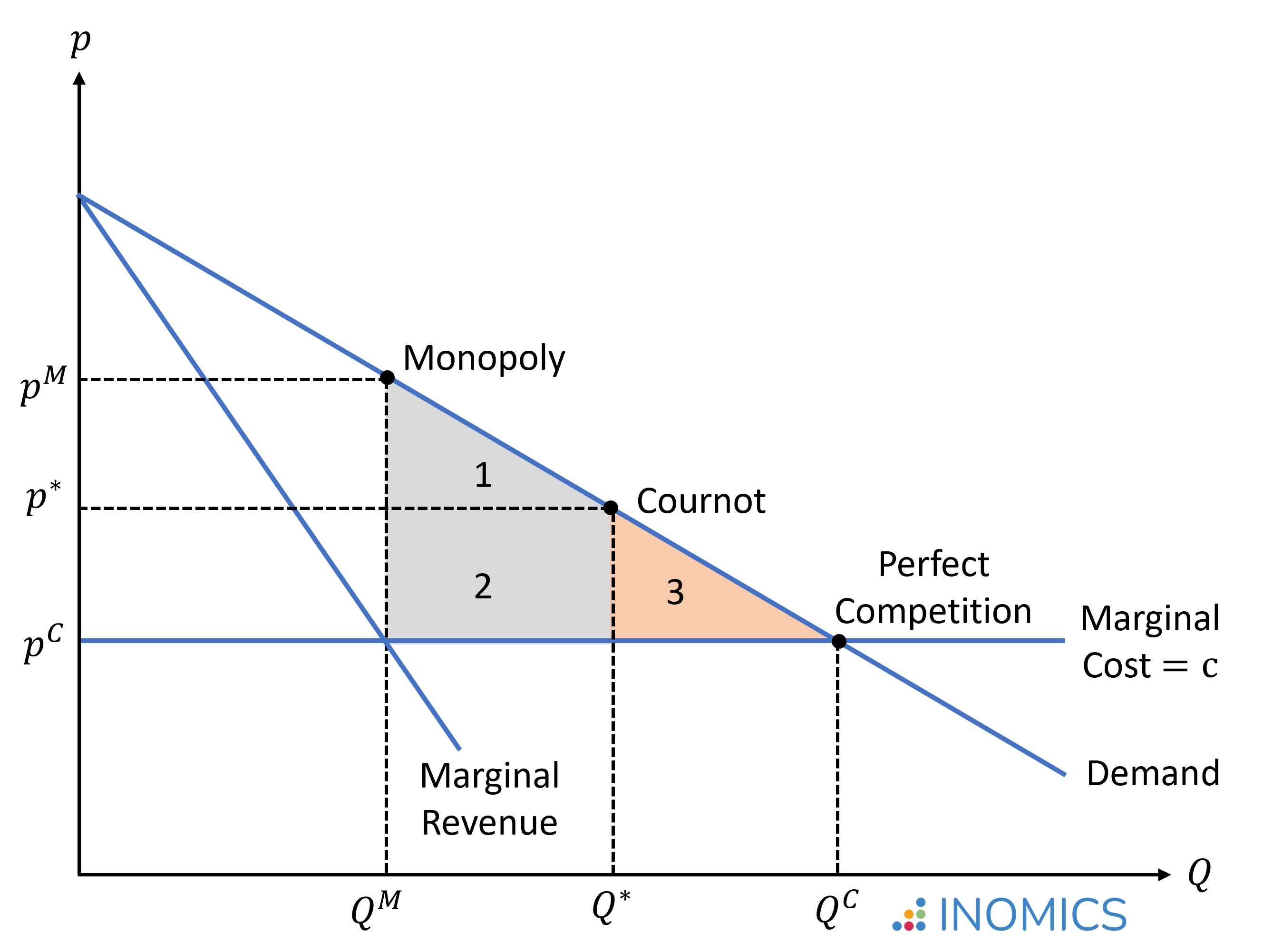
Figure 2: Deadweight loss from a Cournot oligopoly
Good to Know
The Organization of the Petroleum Exporting Countries (OPEC) is often mentioned as a good example of a Cournot oligopoly. Research has shown that the behavior of OPEC member countries is somewhere in between a non-cooperative Cournot oligopoly and a cartel. That is, while there is some cooperation, it can be optimal, especially for smaller OPEC producers (whose production has less potential to impact market prices), to follow more expansionary production policies. The study by Okullo and Reynès (2016) offers interesting insights in this regard.
-
- Assistant Professor / Lecturer Job, Professor Job
- Posted 2 weeks ago
Professor or Associate Professor or Associate Professor (Lecturer) Tenure-track position
At The University of Osaka in Osaka, Japan
-
- Assistant Professor / Lecturer Job
- Posted 1 week ago
Assistant (F/M) in the Research and Teaching Employment Group at Krakow University of Economics
At Krakow University of Economics in 3094802, Poland
-
- Postdoc Job
- Posted 1 week ago
Postdoctoral Research Fellow or Social Science Research Scholar at Stanford (USA) or Heidelberg University (Germany)
At Stanford University in Stanford, United States
Currently trending in United States

Related Items


Upcoming Deadlines
- Jul 29, 2026
- Jul 31, 2026
- Jul 31, 2026
- Aug 01, 2026
- Aug 01, 2026