Economics Terms A-Z
Stackelberg Competition
Read a summary or generate practice questions using the INOMICS AI tool
Stackelberg competition describes an oligopoly market model based on a non-cooperative strategic game where one firm (the “leader”) moves first and decides how much to produce, while all other firms (the “followers”) decide how much to produce afterwards. This sequential structure is the main difference to Cournot’s model, where firms decide simultaneously on the quantities they produce.
The leader might emerge in a market because of its size, reputation, innovative capacity, or because it simply started operating first. The leader will generally be better known and more recognized by customers, and is therefore better placed to decide first which quantity to sell. The follower(s) then decide(s) on their output after observing the leader's production choice.
The Stackelberg leadership model was developed in 1934 by the German economist Heinrich Freiherr von Stackelberg in his book “Market Structure and Equilibrium” (Marktform und Gleichgewicht).
The assumptions in the Stackelberg model are mostly the same as in the Cournot model, with the important exception that firms make their production quantity decisions sequentially. These assumptions are as follows:
- There is a fixed number of firms in the market and firms have market power. This means that each firm's production-decision affects the market price.
- All firms produce a homogenous good, and are subject to the same demand and cost functions. In other words, there is no product differentiation. This means that the goods produced by any firm are completely identical in the eyes of the consumers (they are perfect substitutes).
- Firms compete in terms of the quantities that they produce. That is, they compete for market share. This is the key difference compared to Bertrand competition, in which firms compete in prices.
- Firms decide sequentially on the output they produce, which means we have a model consisting of two distinct periods. In the first period, the leader chooses its production quantity. This decision cannot be changed after. In the second period, the follower firm(s) choose(s) their output after observing the quantity chosen by the leader. This is the key difference when compared to Cournot competition, in which the production decisions by all firms are taken simultaneously.
- Each firm acts strategically on the assumption that its competitor(s) will not change their output, and decides its own production quantity so as to maximize its profit given its competitors’ output.
- Firms do not cooperate.
The Stackelberg-Nash Equilibrium
To derive the Stackelberg-Nash equilibrium, we will focus on the example of a duopoly. That is, there are only two firms in the market. We will assume that firm 1 (leader) and firm 2 (follower) both produce the same good at the same production cost c1 = c2 = c.
We further assume that both firms face the same linear demand function given by:
p(Q) = a - bQ
where a > 0 and b > 0.
The total market quantity is the sum of production by the leader (q1) and the follower (q2), which is Q = q1 + q2. We can substitute this expression for Q in the following equations. Firm 1's total revenue is then given by the market price p(Q) times the quantity produced:
\begin{equation*}
r_1=p(Q)q_1=(a-b(q_1+q_2))q_1 \quad \text{(analogous for firm 2)},
\end{equation*}
and Firm 1's total profits are calculated as the difference between revenue and production costs:
\begin{equation*}
\pi_1= p(Q)q_1-cq_1=(a-b(q_1+q_2)-c)q_1 \quad \text{(analogous for firm 2)}.
\end{equation*}
From here we will assume a > c, which is a necessary condition such that positive profits can be realized.
Each firm chooses the production quantity that maximizes its profits, taking the quantity produced by other firms in the market into consideration. To find the Nash equilibrium of this sequential game, we need to use backward induction. That is, we first solve the optimization problem for the follower in the second period, and with this information determine the optimal choice by the leader in the first period.
In the second period, Firm 2 (follower) chooses q2, taking the quantity produced by the leader in the first period into consideration. So, to derive the optimal output, we need to find the quantity q2 that maximizes the profit function for Firm 2, taking q1 as given. For Firm 2, the problem is thus similar to the Cournot model:
\begin{align*}
\max_{q_2} \{\pi(q_2) &=(a-b(q_1+q_2)-c)q_2\} \\
\frac{\partial \pi(q_2)}{\partial q_2} &= a-bq_1-2bq_2-c = 0 \quad | \quad \text{solve for q2} \\
q_2^* &= R_2(q_1)= \frac{a-bq_1-c}{2b} \quad \text{= Cournot's reaction function}.
\end{align*}
As in the Cournot Model, the equation R2(q1) is the best response function of Firm 2 to any quantity produced by Firm 1.
In the 1st period, Firm 1 (leader) chooses q1, with the understanding that Firm 2 will react to this choice in the second period according to its reaction function R2(q1). To calculate the optimal quantity produced by Firm 1, we thus insert the optimal response of Firm 2 into Firm 1's profit function in place of q2 and then take the first derivative:
\begin{align*}
\max_{q_1} \{\pi(q_1) &=(a-b(q_1+R_2(q_1))-c)q_1=aq_1-bq_1^2-bq_1R_2(q_1)-cq_1\} \\
& \quad \text{Note: Use the product rule to differentiate $-bq_1R_2(q_1)$} \\
\frac{\partial \pi(q_1)}{\partial q_1} &= a-2bq_1-bR_2(q_1)-bq_1R_2'(q1)-c = 0 \quad | \quad \text{insert $R_2$ and $R_2'$} \\
& \Leftrightarrow a-2bq_1-b\left[\frac{a-bq_1-c}{2b}\right]+bq_1\frac{1}{2}-c = 0 \quad | \quad \text{solve for q1} \\
& \Leftrightarrow a-2bq_1-\frac{a}{2}+\frac{bq_1}{2}+\frac{c}{2}+\frac{bq_1}{2}-c=0 \\
& \Leftrightarrow \left[\frac{a-c}{2}\right]-bq_1=0 \\
& \Leftrightarrow q_1^*= \frac{a-c}{2b} > \frac{a-c}{3b} = q_{Cournot}^*.
\end{align*}
Given the quantity produced by the leader, q1*, we can then calculate the output produced by the follower:
\begin{align*}
q_2^* &= \frac{a-bq_1^*-c}{2b} = \left[\frac{a-c}{2b}\right]-q_1^*\frac{1}{2} \quad | \quad \text{insert $q_1^*$} \\
\Leftrightarrow q_2^* &= \left[\frac{a-c}{2b}\right]-\frac{1}{2}\left[\frac{a-c}{2b}\right] \\
\Leftrightarrow q_2^* &= \frac{a-c}{4b} < \frac{a-c}{3b} = q_{Cournot}^*.
\end{align*}
Thus, in the Stackelberg-Nash equilibrium, the leader produces a larger quantity and the follower produces a smaller quantity than the same firms would have produced in the Cournot-Nash equilibrium. The figure below illustrates the difference in quantities produced in a Stackelberg or Cournot oligopoly (imperfect competition) or monopolistic market (firm 1 is the only firm in the market), where q1S > q1C and q2S < q2C:
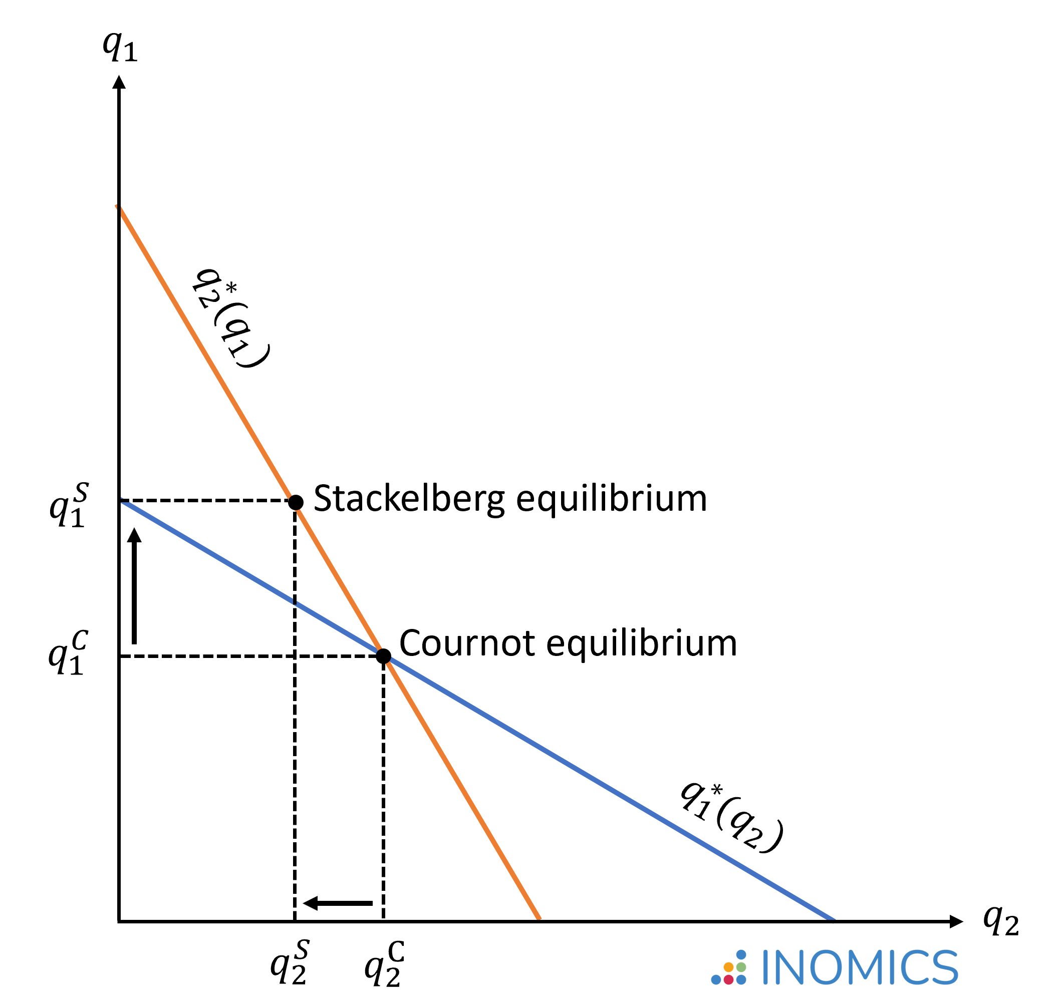
Figure 1: Stackelberg equilibrium compared to Cournot equilibrium
Calculating the total quantity and the market price, given q1* and q2*, we see that Stackelberg's sequential game leads to a more competitive equilibrium -- characterized by a larger total output and lower price level -- than Cournot's simultaneous game:
\begin{align*}
Q^* &= q_1^* + q_2^* = \frac{a-c}{2b} + \frac{a-c}{4b} = \frac{3}{4} \left[\frac{a-c}{b}\right] > \frac{2}{3} \left[\frac{a-c}{b}\right] = Q_{Cournot}^* \\
p^* &= a - bQ^*= a - \frac{3}{4}(a-c) = \frac{a+3c}{4} < \frac{a+2c}{3} = p_{Cournot}^*.
\end{align*}
The Stackelberg leader takes into account that higher output causes the follower to produce less, but also that higher output depresses the price level. In this particular scenario, with a linear demand function and identical costs, the two effects happen to cancel exactly and in this case we end up with a solution where the Stackelberg leader produces the monopoly quantity (although due to the depressed price level, receives less than monopoly profits).
If we were to insert the production quantities and price level into the profit functions, we would find that the Stackelberg leader has higher profits, and the Stackelberg follower lower profits, than the same firms in the Cournot model. This extra profit that the leader has compared to the follower is due to them making a production decision first, which means the follower must accept the leader’s output as given and produce a smaller output for itself. This is called a first mover advantage.
In the figure below, areas 1 + 2 illustrate the welfare gain in the Stackelberg model compared to Cournot model, while area 3 illustrates the remaining deadweight loss compared to a situation of perfect competition. Importantly, the Stackelberg equilibrium is only more efficient than the Cournot equilibrium if firms are symmetric; that is, if both firms have the same production cost. If the leader were to have higher production costs and thus be less efficient than the follower, then the Cournot equilibrium would be preferable from a welfare perspective, since the Stackelberg's sequential model would give an advantage to the less efficient firm with higher costs.
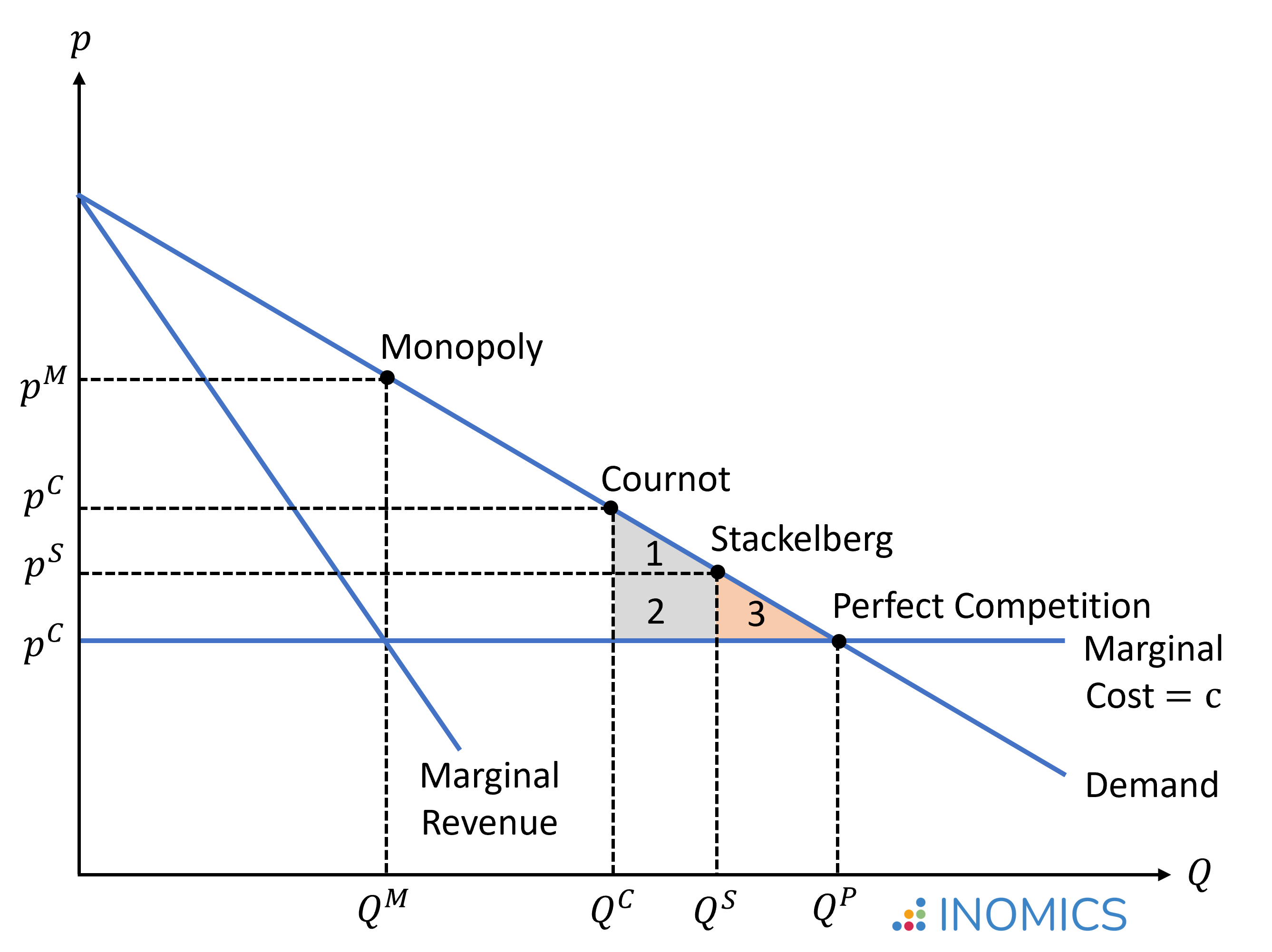
Figure 2: Stackelberg competition surplus compared to Cournot competition and perfect competition
Good to know
Actual markets may exhibit Stackelberg-type competition when, for example, sequential market entry or R&D races put one firm in a better market position than its competitors. Let’s examine Microsoft in the 1990s as an example of this.
Consider the market for operating systems that we use to interact with our computers. Microsoft was the leader in the operating system market in the 1990s, eventually commanding over 90% of market share with their popular Windows OS. Because of this market position, software applications generally needed to be compatible with Microsoft’s operating system. Microsoft’s production decisions overshadowed any following firms, who had to account for the massive market share that Microsoft had (or, devise a plan to capture some of that market share for themselves) when making production decisions.
Eventually Apple computers became popular as well, and the Apple DOS took some market share from Microsoft’s Windows operating systems. Of course, in real life people generally have a strong preference between using a Mac or a PC. This is where the example differs from the Stackelberg model we’ve talked about in this article, since operating systems are not identical in the eyes of consumers. Although the products are similar, in reality there will almost always be some product and price differentiation that causes market dynamics to diverge from the stylized model.
-
- Research Assistant / Technician Job
- Posted 1 week ago
Research Assistant: Foreign and Defense Policy; Demographics and Political Economy
At American Enterprise Institute in Washington, United States
-
- Assistant Professor / Lecturer Job
- Posted 2 weeks ago
Assistant Professor - Economics
At Salisbury University in Salisbury, United States
-
- Event, Conference, PhD Candidate Job
- Posted 6 days ago
Tor Vergata Ph.D. Conference in Economics
At University of Rome Tor Vergata in Rome, Italy
Currently trending in United States


Related Items
-

Visualizing Geospatial Data In Stata: Spatial Maps In Stata - Live Online Course
-

Master in International and Monetary Economics (MIME) - Joint Program by the Universities of Basel and Bern
-
PhD in Economics - University of Pavia & University of Milan - Admission to the 2026/2027 Academic Year (Cycle 42)
Featured Announcements


Upcoming Deadlines
- Jul 21, 2026
- Jul 26, 2026
- Jul 26, 2026
- Jul 29, 2026
- Jul 31, 2026